A knowledge graph is an ever evolving structure. It needs to be extended to be able to cope with new kinds of knowledge; it needs to be fixed and improved in all kinds of different ways. It also needs to be linked to other sources of data and to other knowledge representations such as schemas, ontologies and vocabularies. One of the core tasks related to knowledge graphs is to extend its scope. This idea seems simple enough, but how can we extend a general knowledge graph that has nearly 40,000 concepts with potentially multiple thousands more? How can we do this while keeping it consistent, coherent and meaningful? How can we do this without spending undue effort on such a task? These are the questions we will try to answer with the methods we cover in this article.
The methods we are presenting in this article are how we can extend Cognonto‘s KBpedia Knowledge Graph using an external source of knowledge, one which has a completely different structure than KBpedia and one which has been built completely differently with a different purpose in mind than KBpedia. In this use case, this external resource is the Wikipedia categories structure. What we will show in this article is how we may automatically select the right Wikipedia categories that could lead to new KBpedia concepts. These selections are made using a SVM classifier trained over graph embedding vectors generated by a DeepWalk model based on the KBpedia Knowledge Graph structure linked to the Wikipedia categories. Once appropriate candidate categories are selected using this model, the results are then inspected by a human to take the final selection decisions. This semi-automated process takes 5% of the time it would normally take to conduct this task by comparable manual means.
[extoc]
Extending KBpedia Using Wikipedia Categories
What we want to accomplish is to extend the KBpedia Knowledge Graph by leveraging its own graph structure and its linkage to the external Wikipedia category structure. The goal is to find the sub-graph structure surrounding each of the existing links between these two structures and then to use that graph structure to find new Wikipedia categories that share the same kind of sub-graph structure with KBpedia, but that are not currently linked to any existing KBpedia concept. These candidates could then lead to new KBpedia concepts that are not currently existing in the structure.
The Process
Thousands of KBpedia reference concepts are currently linked to related Wikipedia categories. What we want to do is to use this linkage to propose a series of new sub-classes that we could add to KBpedia based on the sub-categories that exist in Wikipedia for each of these links. What we want to do is to create a list of new KBpedia concepts candidates that comes from the Wikipedia category structure. This new list includes Wikipedia categories that come from:
- The sub-categories of a Wikipedia categories that are linked to a leaf KBpedia reference concept,
- The sub-categories of a Wikipedia categories that are linked to a KBpedia reference concept which is the parent of a leaf concept, and
- The sub-categories of a Wikipedia categories that are linked to a KBpedia reference concept which is not
1.nor2.
The idea is that 1. and 2. would use the Wikipedia category structure to specialize the KBpedia conceptual structure and 3. would fix potential scope/coverage of the structure with new general concepts.
The challenge we face by proceeding in this way is that our procedure potentially creates tens of thousands of new candidates. Because the Wikipedia category structure has a completely different purpose than the KBpedia Knowledge Graph, and because Wikipedia’s creation rules are completely different than KBpedia, many candidates are inconsistent or incoherent to include in KBpedia. Most of the candidate categories need to be dropped. Reviewing hundred of thousands of new candidates manually is not tenable without an automatic way to rank potential candidates.
An objective of the process is to greatly reduce the cost of such an Herculean task by using machine learning techniques to help the human reviewer by pre-categorizing each of the proposed new sub-class-of relationships.
We thus problem split the problem into three distinct tasks:
- The first thing we have to do is to learn the sub-category patterns that exists in the Wikipedia category structure. These patterns will be learned in an unsupervised manner using the DeepWalk algorithm. Graph embedding vectors will be created from this task;
- Then we create a training set with thousands of pre-classified sub-categories.
75%of the training set is used for training, and25%of it is used for cross-validation. The classifier we will use for this task is SVM with a RBF kernel; and - Employ hyper parameter optimization of the previous 2 steps.
Once these three steps are completed, we will classify all of the proposed sub-categories and create a list of potential sub-class-of candidates to add into KBpedia, which is then validated by a human. These steps should significantly reduce the time required to add new reference concepts using an external structure such as the Wikipedia category structure.
Cleaning Wikipedia Categories
KBpedia presently links to what we call the “clean” categories within the Wikipedia category structure. These same “clean” categories are used by this present article.
The reason for “cleaning” the Wikipedia categories is to remove internal administrative categories of use to Wikipedia alone and to remove “compound” or “artificial” categories frequently found in Wikipedia that do not conform to natural classes but are matters of grouping convenience (such as Films directed by Pedro Almodóvar or Ambassadors of the United States to Mexico).
The process that creates this “clean” category listing for Wikipedia consists of the following is:
- Read all Wikipedia categories,
- Remove all administrative categories that were collected by hand inspection,
- Remove all articles related categories that were collected by hand inspection,
- Remove all dates related categories that were collected by hand inspection,
- Remove all categories that had some preposition patterns that were collected by hand inspection,
- Remove all the lists categories that were collected by hand inspection, and
- Remove other categories that were tagged to be removed that do not fall into any categories listed above.
The result of this category filtering process is to produce a “clean” list of 88,691 Wikipedia categories. Note this is a significant reduction for the total category listing found on Wikipedia itself. This list is also what is used as input to the Cognonto Mapper service, which is what is used as the candidate pool for possible matches between any of these clean Wikipedia categories and existing KBpedia reference concepts. Final selections, wherever made, are drawn from this “clean” candidate pool and vetted by a human prior to acceptance.
Introducing DeepWalk
DeepWalk was created to learn social representations of a graph’s vectices that capture neighborhood similarity and community membership. DeepWalk generalizes neural language models to process a special language composed of a set of randomly-generated walks.
With Cognonto, we want to use DeepWalk not to learn social representations but to learn the relationship (that is, the similarity) between all of the concepts existing in a Knowledge Graph given different kinds of relationships such as sub-class-of, super-class-of, equivalent-class or other relationships such as KBpedia’s 80 aspects relationships.
For this use case we use the DeepWalk algorithm to select concepts from an external conceptual structure that could be added into the KBpedia Knowledge Graph that shares the same graph structure. Other tasks that could be performed using DeepWalk in a similar manner are:
- Content recommendation,
- Anomaly detection [in the Knowledge Graph], or
- Missing link prediction [in the Knowledge Graph].
Note that we randomly walk the graphs as stated in DeepWalk’s original paper 1. However more experiments could be performed to change the random walk by other graph walk strategies like depth-first or breadth-first walks.
Finding Candidates
The first step we have to do is to find all of the potential Wikipedia category cadidates that could become new KBpedia reference concepts based on their graph structure. What we have to do is to list all these candidates according to this heuristic:
- The sub-categories of a Wikipedia categories that are linked to a leaf KBpedia reference concept,
- The sub-categories of a Wikipedia categories that are linked to a KBpedia reference concept which is the parent of a leaf concept,
- The sub-categories of a Wikipedia categories that are linked to a KBpedia reference concept which is not
1.nor2.
Each of these steps will lead to a different list of candidates.
The first step is to load the KBpedia Knowledge Graph to analyze its leaf, near-leaf and core concepts structure:
(require '[cognonto-owl.model :as model])
(require '[cognonto-owl.query :as query])
(require '[cognonto-owl.core :as owl])
(require '[cognonto-owl.reasoner :as reasoner])

(def onto-iri (str "file:/d:/cognonto-git/cognonto-deepwalk/resources/kbpedia_reference_concepts.n3"))
(def kbpedia-manager (owl/make-ontology-manager))
(def kbpedia (owl/load-ontology onto-iri :ontology-manager kbpedia-manager))
(def kbpedia-reasoner (reasoner/make-reasoner kbpedia))
(defn is-near-leaf?
  "Return true is the reference concept is a leaf or is the parent of a leaf concept
   of the graph."
  ([rc]
   (is-near-leaf? rc 1))
  ([rc depth]
   (let [sub-classes (query/sub-classes rc kbpedia :direct true)]
     (if (empty? sub-classes)
       true
       (if (= 0 depth)
         false
         (->> sub-classes
              (map (fn [sub-class]
                     (is-near-leaf? sub-class (dec depth))))
              (apply = true)))))))

(defn is-leaf?
  "Return true is the reference concept is a leaf concept in the graph."
  [rc]
  (if (empty? (query/sub-classes rc kbpedia :direct true))
    true
    false))
Then we create the three lists of KBpedia reference concepts:
(def near-leaf-rcs (->> (query/get-classes kbpedia)
                        (map (fn [rc]
                               (when (is-near-leaf? rc)
                                 (when-not (is-leaf? rc)
                                   rc))))
                        (remove nil?)
                        (into [])))

(def leaf-rcs (->> (query/get-classes kbpedia)
                   (map (fn [rc]
                          (when (is-leaf? rc)
                            rc)))
                   (remove nil?)
                   (into [])))

(def core-rcs (->> (query/get-classes kbpedia)
                   (map (fn [rc]
                          (when-not (is-near-leaf? rc)
                            rc)))
                   (remove nil?)
                   (into [])))
Each of these lists is composed of the following number of reference concepts:
(println "Leaf reference concepts: " (count leaf-rcs))
(println "Near-leaf reference concepts: " (count near-leaf-rcs))
(println "Core reference concepts: " (count core-rcs))
Finally what we do is to query the Wikipedia category structure to get the list of all the sub-categories linked to each of the leaf, near-leaf and core KBpedia reference concepts. We serialize this list of candidates into 3 distinct CSV files.
(get-immediate-sub-categories leaf-rcs "resources/leaf-rcs-narrower-concepts.csv")
(get-immediate-sub-categories near-leaf-rcs "resources/near-leaf-rcs-narrower-concepts.csv")
(get-immediate-sub-categories core-rcs "resources/core-rcs-narrower-concepts.csv")
Each of these lists leads to 34,957 leaf categories candidates, 6,104 near-leaf categories candidates and 6,066 core categories candidates for a grand total of 47,127 new KBpedia reference concept candidates to review.
Create Graph Embedding Vectors
The next step is to create the graph embedding for each of the Wikipedia categories. What we have to do is to use the Wikipedia category structure along with the linked KBpedia Knowledge Graph. Then we have to generate the graph embedding for each of the Wikipedia categories that exists in the structure.
The graph embeddings will be generated using the DeepWalk algorithm over that linked structure. It will randomly walk the linked graph hundred of times to generate the graph embeddings for each category.
Create Deeplearning4j Graph
To generate the graph embeddings, we will use Deeplearning4j’s DeepWalk implementation. The first step is to create a Deeplearning4j graph structure that will be used by its DeepWalk implementation to generate the embeddings.
The graph we have to create is composed of the latest version of the Wikipedia category structure along with the latest version of the KBpedia Knowledge Graph. The Wikipedia category structure comes from the DBpedia file 2015-10slcore-i18nslenslskoscategoriesen.ttl.bz2 and the KBpedia Knowledge Graph version 1.20.
Because of the size of the file, we will simply read the Turtle file and create the vertices and the edges in the graph on the fly with some regular expression operations on each line. In the process, we will create two intermediary CSV files: one that lists all the edges, and one that lists all the vertices used to create the Deeplearning4j graph structure:
(import org.deeplearning4j.graph.graph.Graph)
(import org.deeplearning4j.graph.api.Vertex)
(import org.deeplearning4j.graph.models.deepwalk.DeepWalk$Builder)
(require '[clojure.java.io :as io])
(require '[clojure.data.csv :as csv])

(defn create-dl4j-graph-vertices-index-csv
  [n3-file csv-file & {:keys [base-uri]
                       :or {base-uri nil}}]
  (with-open [in-file (io/reader n3-file)]
    (with-open [out-file (io/writer csv-file)]
      (doseq [vertice (->> (line-seq in-file)
                           (mapcat (fn [line]
                                     (when-let [matches (re-matches #"^<.*resource/Category:(.*?)>.*<.*broader.*>.*<.*resource/Category:(.*)>.*$" line)]
                                       [(nth matches 1)
                                        (nth matches 2)])))
                           (distinct)
                           (sort)
                           (into []))]
        (csv/write-csv out-file [[(if-not (nil? base-uri)
                                    (str base-uri vertice)
                                    vertice)]])))))

(defn create-dl4j-graph-edges-index-csv
  [n3-file csv-file & {:keys [base-uri]
                       :or {base-uri nil}}]
  (with-open [in-file (io/reader n3-file)]
    (with-open [out-file (io/writer csv-file)]
      (doseq [line (line-seq in-file)]
        (when-let [matches (re-matches #"^<.*resource/Category:(.*?)>.*<.*broader.*>.*<.*resource/Category:(.*)>.*$" line)]
          (csv/write-csv out-file [[(if-not (nil? base-uri)
                                      (str base-uri (nth matches 1))
                                      (nth matches 1))
                                    (if-not (nil? base-uri)
                                      (str base-uri (nth matches 2))
                                      (nth matches 2))]]))))))
Now we will generate the two intermediary CSV files:
(create-dl4j-graph-vertices-index-csv "resources/skos_categories_en.ttl"
                                      "resources/skos_categories_vertices.csv"
                                      :base-uri "http://wikipedia.org/wiki/Category:")

(create-dl4j-graph-edges-index-csv "resources/skos_categories_en.ttl"
                                   "resources/skos_categories_edges.csv"
                                   :base-uri "http://wikipedia.org/wiki/Category:")
Finally we will generate the initial Deeplearning4j graph structure composed of the Wikipedia category structure and the inferred KBpedia Knowledge Graph. The resulting linked structure will compose the graph used by the DeepWalk algorithm to generate the embedding vectors for each of the Wikipedia categories.
(require '[cognonto-owl.core :as owl])
(require '[cognonto-owl.reasoner :as reasoner])

(def onto-iri (str "file:/d:/cognonto-git/cognonto-deepwalk/resources/kbpedia_reference_concepts_linkage_inferrence_extended.n3"))
(def kbpedia-manager (owl/make-ontology-manager))
(def kbpedia-graph (owl/load-ontology onto-iri :ontology-manager kbpedia-manager))
(def kbpedia-reasoner (reasoner/make-reasoner kbpedia-graph))
(defn create-deepwalk-graph-from-wikipedia-categories-and-kbpedia
  [vertices-file edges-file knowledge-graph & {:keys [directed?]
                                               :or {directed? true}}]
  (let [index (->> (into (->> (query/get-classes knowledge-graph)
                              (mapv (fn [class]
                                      (.toString (.getIRI class)))))
                         (->> (with-open [in-file (io/reader vertices-file)]
                                (doall
                                 (csv/read-csv in-file)))
                              (mapv (fn [[class]]
                                      class))))
                   distinct
                   (map-indexed (fn [i vertice]
                                  {vertice (inc i)}))
                   (apply merge))
        index (merge {"http://www.w3.org/2002/07/owl#Thing" 0} index)
        index (into (sorted-map-by (fn [key1 key2]
                                     (compare [(get index key1) key1]
                                              [(get index key2) key2]))) index)
        graph (new Graph (mapv (fn [[class i]] (new Vertex i class)) index) false)]

        (doseq [[vertice-1 vertice-2] (with-open [in-file (io/reader edges-file)]
                                        (doall
                                         (csv/read-csv in-file)))]
          (.addEdge graph (get index vertice-1) (get index vertice-2) "sub-class-of" directed?))

        (doseq [class (query/get-classes knowledge-graph)]
          (doseq [super-class (query/super-classes class knowledge-graph :direct true :reasoner kbpedia-reasoner)]
            (try
              (.addEdge graph (get index (.toString (.getIRI class))) (get index (.toString (.getIRI super-class))) "sub-class-of" directed?)
              (catch Exception e))))

        ;; Make sure that all the nodes are at least connected to owl:Thing
        (doseq [i (take (.numVertices graph) (iterate inc 0))]
          (when (<= (.getVertexDegree graph i) 0)
            (.addEdge graph i 0 "sub-class-of" directed?)))

        graph))
Now let’s generate the final Deeplearning4j graph that will be used by the DeepWalk algorithm to generate the Wikipedia categories graph embeddings.
(def graph (create-deepwalk-graph-from-wikipedia-categories-and-kbpedia "resources\\skos_categories_vertices.csv"
                                                                        "resources\\skos_categories_edges.csv"
                                                                        kbpedia-graph
                                                                        :directed? true))
Train DeepWalk
Once the Deeplearning4j graph is created, the next step is to create and train the DeepWalk algorithm. What the (create-deep-walk) function does is to create and initialize a DeepWalk object with the Graph we created above and with some hyperparameters.
The :window-size hyperparameter is the size of the window used by the continuous Skip-gram algorithm used in DeepWalk. The :vector-size hyperparameter is the size of the embedding vectors we want the DeepWalk to generate (it is the number of dimensions of our model). The :learning-rate is the initial leaning rate of the Stochastic gradient descent.
For this task, we initially want to have a window of 15, 3 dimensions to initially make visualizations simpler to interpret, and an initial learning rate of 2.5%.
(use '[cognonto-deepwalk.core])

(def deep-walk (create-deep-walk graph
                                 :window-size 15
                                 :vector-size 3
                                 :learning-rate 0.025))
Once the DeepWalk object is created and initialized with the graph, the next step is to train that model to generate the embedding vectors for each vertice in the graph.
The training is performed using a random walk iterator. The two hyperparameters related to the training process are the walk-length and the walks-per-vertex. The walk-length is the number of vertices we want to visit for each iteration. The walks-per-vertex is the number of timex we want to create random walks for each vertex in the graph.
(defn train
  ([deep-walk iterator]
   (train deep-walk iterator 1))
  ([deep-walk iterator walks-per-vertex]
   (.fit deep-walk iterator)
   (dotimes [n walks-per-vertex]
     (.reset iterator)
     (.fit deep-walk iterator)))
  ([deep-walk graph walk-length walks-per-vertex]
   (train deep-walk (new RandomWalkIterator graph walk-length) walks-per-vertex)))
For the initial setup, we want to have a walk-lenght of 15 and we want to iterate the process 175 times per vertex.
(train deep-walk graph 15 175)
Create Training Sets
Now that the DeepWalk algorithm has been created and trained, we will now create the training sets that will be used to create the SVM classification model. The training set is created from the manually vetted linkages between the KBpedia Knowledge Graph and the Wikipedia category structure. 75% of the vetted linkages will be used for training and 25% for cross validation. This sampling is performed randomly.
(defn build-svm-model-vectors
  "Build the vectors used to train the SVM model that is used to determine
   if a sub-category is likely to create a good new reference concept
   candidate based on its graph embedding vector."
  [training-set-csv-file deep-walk index & {:keys [base-uri]
                                            :or {base-uri nil}}]
  (let [training-csv (rest
                      (with-open [in-file (io/reader training-set-csv-file)]
                        (doall
                         (csv/read-csv in-file))))
        sets (->> training-csv
                  (map (fn [[kbpedia-rc wikipedia-category possible-new-sub-class-of is-sub-class-of?]]
                         (when (and (not (empty? possible-new-sub-class-of))
                                    (not (nil? (get index (if (nil? base-uri)
                                                            possible-new-sub-class-of
                                                            (str base-uri possible-new-sub-class-of))))))
                           (list {:name possible-new-sub-class-of
                                  :class (if (= is-sub-class-of? "x")
                                           1
                                           0)
                                  :f (into (sorted-map-by <)
                                           (->> (read-string
                                                 (.toString
                                                  (.data
                                                   (.getVector (.lookupTable deep-walk)
                                                               (get index (if (nil? base-uri)
                                                                            possible-new-sub-class-of
                                                                            (str base-uri possible-new-sub-class-of)))))))
                                                (map-indexed (fn [feature-id value]
                                                               {feature-id value}))
                                                (apply merge)))}))))
                  (apply concat)
                  (remove nil?))
        sets (shuffle sets)
        sets (split-at (int (java.lang.Math/floor (* (count sets) 0.75))) sets)]
    {:training (first sets)
     :validation (second sets)}))
(def model-vectors (build-svm-model-vectors "resources/core-wikipedia-subclass-mapped--extended.csv"
                                            deep-walk
                                            index
                                            :base-uri "http://wikipedia.org/wiki/Category:"))
The training set is composed of 7,124 items and the validation set is composed of 2,375. There are 7,646 positive training examples and 1,853 negative ones.
Train SVM Classifier
Now that the training and the validation sets have been generated, the next step is to train the SVM classifier using the training set. The initial evaluation of our model will use the following hyperparameters values. Also, the SVM implementation we use is LIBSVM implemented in Java. We use the RBF kernel.
(use 'svm.core)

(def libsvm-model (svm.core/train-model (->> (:training model-vectors)
                                             (map (fn [item]
                                                    [(if (= (:class item) 0)
                                                       -1
                                                       1)
                                                     (->> (:f item)
                                                          (map (fn [[k v]]
                                                                 {(inc k) v}))
                                                          (apply merge))]))
                                             concat)
                                        :eps 1e-3
                                        :gamma 0
                                        :kernel-type (:rbf svm.core/kernel-types)
                                        :svm-type (:one-class svm.core/svm-types)))
Evaluate Model
Once the SVM model is trained, the next step is to evaluate its performance. The different performance metrics are calculate using the following function:
(defn evaluate-libsvm-model
  [model-vectors svm-model]
  (let [validation-set (:validation model-vectors)
        true-positive (atom 0)
        false-positive (atom 0)
        true-negative (atom 0)
        false-negative (atom 0)]
    (doseq [case validation-set]
      (let [predicted-class (svm.core/predict svm-model (:f case))]
        (when (and (= (:class case) 1)
                   (= predicted-class 1.0))
          (swap! true-positive inc))

        (when (and (= (:class case) 0)
                   (= predicted-class 1.0))
          (swap! false-positive inc))

        (when (and (= (:class case) 0)
                   (= predicted-class -1.0))
          (swap! true-negative inc))

        (when (and (= (:class case) 1)
                   (= predicted-class -1.0))
          (swap! false-negative inc))))

    (println "True positive: " @true-positive)
    (println "false positive: " @false-positive)
    (println "True negative: " @true-negative)
    (println "False negative: " @false-negative)
    (println)

    (if (= 0 @true-positive)
      (let [precision 0
            recall 0
            accuracy 0
            f1 0]

        (println "Precision: " precision)
        (println "Recall: " recall)
        (println "Accuracy: " accuracy)
        (println "F1: " f1)

        {:precision precision
         :recall recall
         :accuracy accuracy
         :f1 f1})
      (let [precision (float (/ @true-positive (+ @true-positive @false-positive)))
            recall (float (/ @true-positive (+ @true-positive @false-negative)))
            accuracy (float (/ (+ @true-positive @true-negative) (+ @true-positive @false-negative @false-positive @true-negative)))
            f1 (float (* 2 (/ (* precision recall) (+ precision recall))))]

        (println "Precision: " precision)
        (println "Recall: " recall)
        (println "Accuracy: " accuracy)
        (println "F1: " f1)

        {:precision precision
         :recall recall
         :accuracy accuracy
         :f1 f1}))))
(evaluate-libsvm-model model-vectors libsvm-model)
True positive:  1000
false positive:  207
True negative:  227
False negative:  941

Precision:  0.8285004
Recall:  0.51519835
Accuracy:  0.5166316
F1:  0.635324
SVM Hyperparameters Optimization
The last step is to optimize the hyperparameters of the prediction workflow. A grid search algorithm is used to optimize the following SVM hyperparameters that uses a RBF kernel with the one-class algorithm:
gamma,eps,- Usage of
shrinking, and - Usage of
probability
This algorithm simply iterates over all of the possible combinations of hyperparameter values as specified in the input grid parameters.
(defn svm-grid-search-one-class-rbf
  [model-vectors & {:keys [grid-parameters selection-metric]
                    :or {grid-parameters [{:gamma [1 1/2 1/3 1/4 1/5 1/7 1/10 1/50 1/100]
                                           :eps [0.000001 0.00001 0.0001 0.001 0.01 0.1 0.2]
                                           :nu [0.1 0.2 0.3 0.4 0.5 0.6 0.7 0.8 0.9]
                                           :probability [0 1]
                                           :shrinking [0 1]
                                           :selection-metric :f1}]}}]
  (let [best (atom {:score 0.0
                    :eps nil
                    :nu nil
                    :gamma nil
                    :probability nil
                    :shrinking nil})
        training-vector (->> (:training model-vectors)
                             (map (fn [item]
                                    [(if (= (:class item) 0)
                                       -1
                                       1)
                                     (->> (:f item)
                                          (map (fn [[k v]]
                                                 {(inc k) v}))
                                          (apply merge))]))
                             concat)]
    (doseq [parameters grid-parameters]
      (doseq [probability (:probability parameters)]
        (doseq [shrinking (:shrinking parameters)]
          (doseq [gamma (:gamma parameters)]
            (doseq [nu (:nu parameters)]
              (doseq [eps (:eps parameters)]
                (let [svm-model (svm.core/train-model training-vector
                                                      :eps eps
                                                      :gamma gamma
                                                      :nu nu
                                                      :shrinking shrinking
                                                      :probability probability
                                                      :kernel-type (:rbf svm.core/kernel-types)
                                                      :svm-type (:one-class svm.core/svm-types))
                      results (evaluate-libsvm-model model-vectors svm-model)]
                  (println "Probability:" probability)
                  (println "Shrinking:" shrinking)
                  (println "Gamma:" gamma)
                  (println "Eps:" eps)
                  (println "Nu:" nu)
                  (println)

                  (when (> (get results (:selection-metric parameters)) (:score @best))
                    (reset! best {:score (get results (:selection-metric parameters))
                                  :gamma gamma
                                  :eps eps
                                  :nu nu
                                  :probability probability
                                  :shrinking shrinking})))))))))
      @best))
Let’s run the grid search to find the best values for each of the hyperparameters of the SVM classifier that uses a RBF kernel while optimizing the result of the F1 score.
(svm-grid-search-one-class-rbf model-vectors :grid-parameters [{:gamma [1 1/2 1/3 1/4 1/5 1/7 1/10 1/50 1/100]
                                                                :eps [0.000001 0.00001 0.0001 0.001 0.01 0.1 0.2]
                                                                :nu [0.1 0.2 0.3 0.4 0.5 0.6 0.7 0.8 0.9]
                                                                :probability [0 1]
                                                                :shrinking [0 1]
                                                                :selection-metric :f1}])
Finally let’s create the final optimized SVM model that uses these optimal hyperparameters.
(def libsvm-model-optimized (svm.core/train-model (->> (:training model-vectors)
                                                       (map (fn [item]
                                                              [(if (= (:class item) 0)
                                                                 -1
                                                                 1)
                                                               (->> (:f item)
                                                                    (map (fn [[k v]]
                                                                           {(inc k) v}))
                                                                    (apply merge))]))
                                                       concat)
                                                  :eps 0.2
                                                  :gamma 1
                                                  :probability 0
                                                  :shrinking 0
                                                  :nu 0.1
                                                  :kernel-type (:rbf svm.core/kernel-types)
                                                  :svm-type (:one-class svm.core/svm-types)))
Visualize With TensorFlow Projector
What we want want to do next is to visualize the apparent “relationship” between each of the positive and negative training examples based on their latent representation vectors as computed by the DeepWalk algorithm. We will visualize the training set using two different methods: Principal Component Analysis (PCA) and t-distributed Stochastic Neighbor Embedding (t-SNE).
The goal of trying to visualize the graph using these techniques is to try to find insights into the models we created and see if our intuition holds.
Note that the following visualizations are used to get insights into the model(s) we are trying to create. The visualizations help find possible correlations, boundaries and outliners in the model. By the nature of the algorithms used, these visualizations should not be overinterpreted. It is to be noted that “The assumption that the data lies along a low-dimentional manifold may not always be correct or useful. We argue that in the context of AI tasks, such as those that involve processing images, sounds, or text, the manifold assumption is at least approximately correct.” 2
The tool we use to create these visualizations is the TensorFlow Projector web application. This visualization tool requires two input CSV files: one which lists all the vertices of the graph with their embedding vectors, and one that lists all metadata (name, class, etc.) of each of these vertices.
(defn generate-tensorflow-projector-vectors-libsvm
  [model-vectors svm-model vectors-file-name metadata-file-name]
  (with-open [out-file-vectors (io/writer (str "resources/" vectors-file-name))]
    (with-open [out-file-metadata (io/writer (str "resources/" metadata-file-name))]
      (csv/write-csv out-file-metadata [["name" "class"]] :separator \tab)
      (doseq [model (:training model-vectors)]
        (csv/write-csv out-file-vectors [(into [] (vals (:f model)))] :separator \tab)
        (csv/write-csv out-file-metadata [[(:name model) "n/a"]] :separator \tab))
      (doseq [model (:validation model-vectors)]
        (csv/write-csv out-file-vectors [(into [] (vals (:f model)))] :separator \tab)
        (csv/write-csv out-file-metadata [[(:name model) (if (= (svm.core/predict svm-model (:f model)) 1.0)
                                                           1
                                                           0)]] :separator \tab)))))
(generate-tensorflow-projector-vectors-libsvm model-vectors
                                              libsvm-model-optimized
                                              "kbpedia-projector-vectors-libsvm-optimized.csv"
                                              "kbpedia-projector-metadata-libsvm-optimized.csv")
Principal Component Analysis
PCA can be viewed as an unsupervised learning algorithm that learns the representation of data: to identify patterns in data, so to detect correlations between variables. Before starting to look into these visualization and to try to get insights from them, let’s review how they get created in the first place.
Each node in the scatter plots below are concepts that belong to the training and validation sets. Their positioning in the plot is determined by their graph embeddings. Their graph embeddings are the latent representation of the concept within the graph composed of the KBpedia Knowledge Graph linked to the Wikipedia categories. Then what we did is to generate meta-data for each of these nodes. The meta-data is composed of two things:
- The name of the concept we consider adding to the KBpedia Knowledge Graph that comes from the Wikipedia category,
- The SVM classification for each of these concepts. The SVM classification can one one of three values:
0– which means that the node doesn’t belong to the class,1– which means that the node does belong to the class, orn/a– which means that the node belong to the training set. Note that only the validation set is classified by the SVM.
The SVM classification of each of these nodes is unrelated to the way the PCA or the t-SNE algorithms will present the graph. However we want to see if there are some correlations between the two by checking the positioning of the nodes given how the SVM classified them.
All the scatter plots below have been generated using TensorFlow’s Projector application. For each of them, we also link the vectors, metadata and bookmark that will enable you to visualize the same graph in the Projector and that will enable you to manipulate and explore these graphs further.
To load this scatter plot, download this package, to do http://projector.tensorflow.org/, then load the vectors and metadata files. Finally load the bookmark using the txt file from the package.
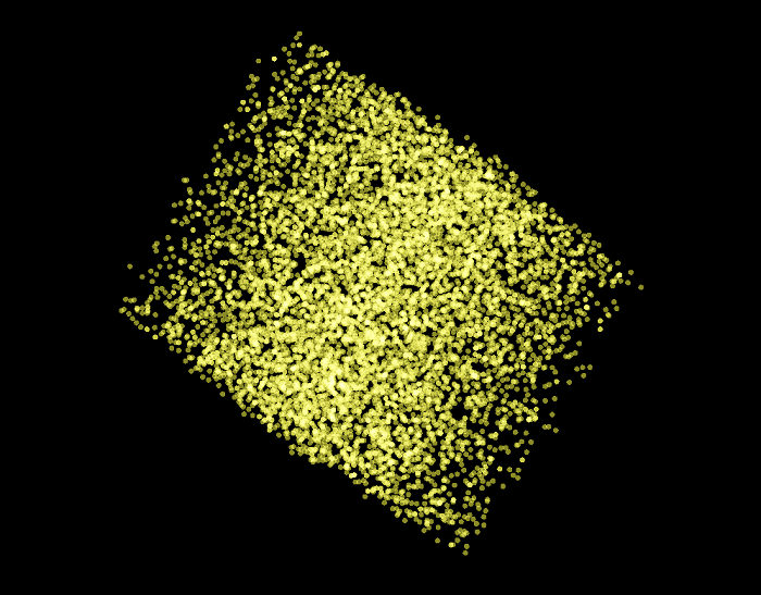
In the following scatter plot, we can see all the 9,499 examples of the training and validation sets as visualized by the PCA algorithm.
Now we only highlight the negative examples of the validation set. What we can observe in this graph is that all the examples that have been classified by the SVM model we created above have been displayed at the edges of the PCA plot.
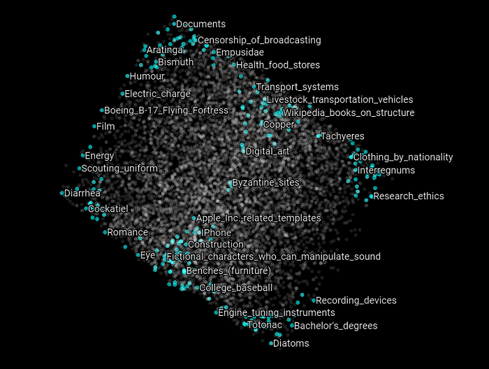
Then if we highlight the positive examples of the validation set, we can observe that all the examples that have been classified by the SVM model have been arranged at the center of the PCA plot.

What this suggests is that some kind of structure emerged from the creation of the graph embedding, how they got classified using the training set, and they got classified by the SVM classifier and how they got arranged by the PCA algorithm. Let’s investigate further with the t-SNE algorithm.
t-distributed Stochastic Neighbor Embedding
t-SNE is another unsupervised learning algorithm that tries to learn the representation of the data to get insights about it. In the following graphs, we will see a few 3-dimensional scatter plots to see what they look like, but we will focus on the 2-dimensional renderings of the same plots since they will be easier to visualize and interpret in this article. We encourage you to load the graphs in the TensorFlow Projector to play with and manipulate the 3-dimensional expressions of the plot.
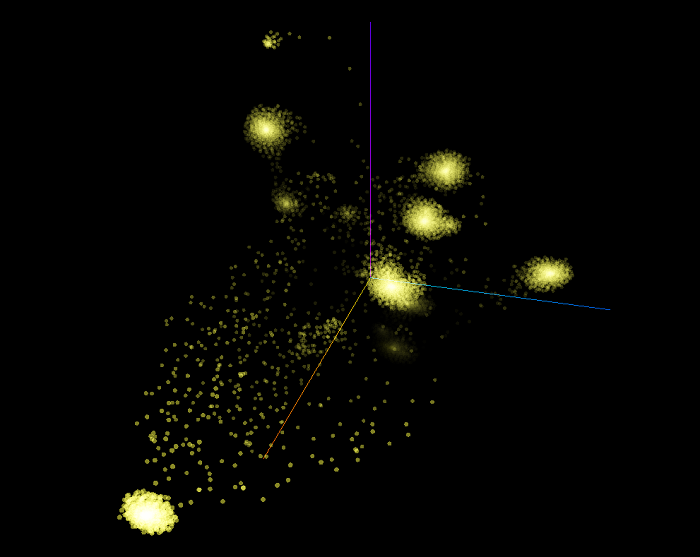
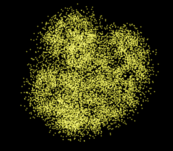
The following 3D scatter plot shows all the 9,499 examples from the training and the validation sets as rendered by the t-SNE algorithm. This graph used a perplexity of 25, a learning rate of 10 and we ran the algorithm for 8,500 iterations. Remember that the graph embedding vectors of these examples have 3 features, which means that they are represented in 3 dimensions. However, when we will visualize the same t-SNE graphs in 2 dimensions, the dimension will be reduced by 1 by the algorithm.
What we can observe is that a few big clusters emerged. Theoretically, the features learned by the DeepWalk algorithm represent the inner structure of the graph surrounding the vertices (concepts). With the current graph we created, we have the full KBpedia Knowledge Graph structure linked to the full Wikipedia category structure. These cluster should represent concepts that have a similar graph structures when we the DeepWalk algorithm randomly walk each vertex following the sub-class-of directed edges of the graph up to depth of 15.
Intuitively we assume that these clusters are created because they are following a similar conceptual parental chain up to shared SuperTypes.
Now let’s highlight the negative examples of the validation set. What we can observe in this graph is that all the examples that have been classified by the SVM model we created above have been displayed at the center of each cluster created by the t-SNE algorithm.
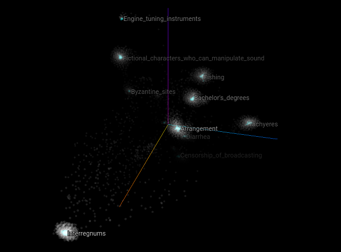
When highlighting the positive examples of the validation set, we can see that almost all of the vertices belong to the clusters, but apparently the outer edges of the clusters.
Now let’s reduce the number of dimensions to two dimensions to have an overall easier scatter plot to visualize. Here are all the training and validation set examples.
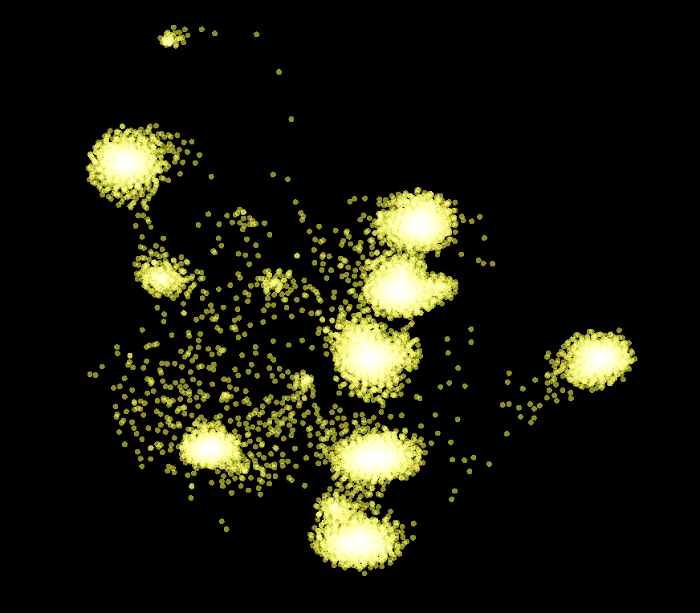
Here we only focus on the negative examples of the validation set. We can clearly see that each of the negative examples appears at the center of each cluster.
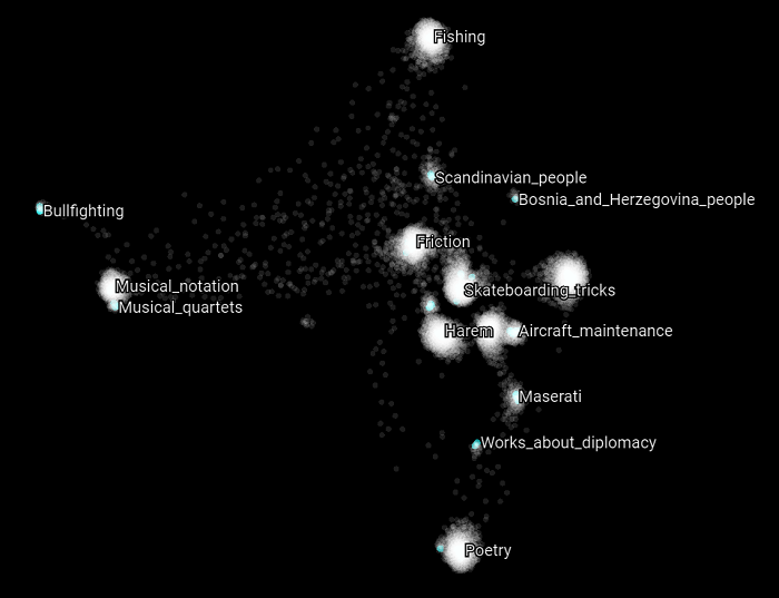
Here we only focus on the positive examples of the validation set.

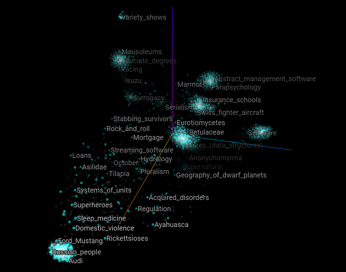
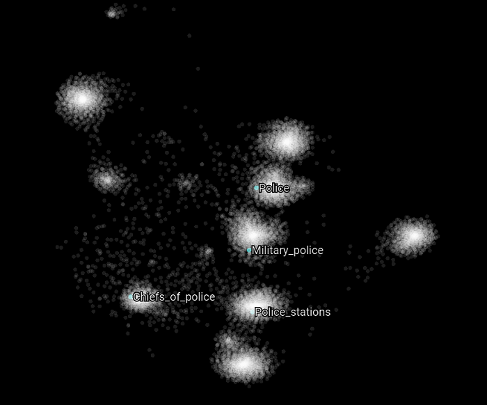
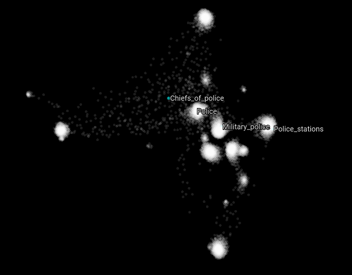
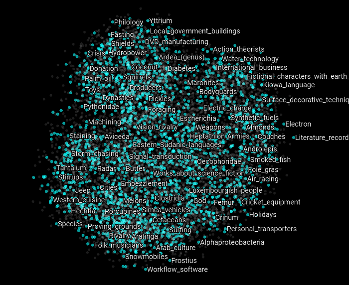
Now let’s focus on specific Wikipedia categories that can belong to the training or the validation set. In the following scatter plot, we highlight all the categories that have the word “police” in them. What we can observe is that each of these categories related to the general topic police belong to different clusters. But at the same time, they refer to different kinds of concepts related to the police topic. What this suggests and may validate is that the intuition we had about the nature of these clusters is that they are related to some SuperType and that they are clustered as such. Let’s see if this holds with other kind of topics as well.
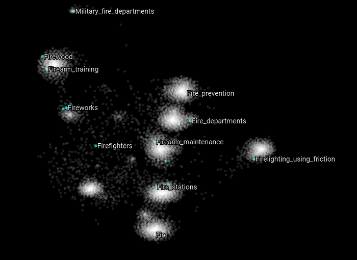
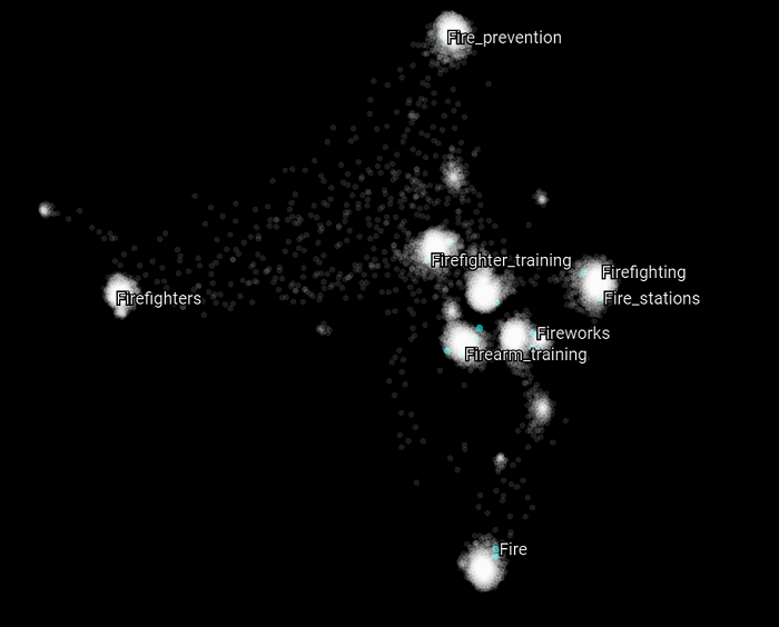
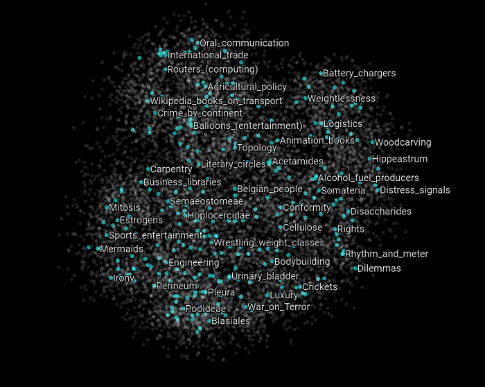
Here we highlight all the Wikipedia categories that have the word “fire” in them. The same appears to be happening again. Most of the concepts belongs to distinct clusters and appears to be related to different upper structure concepts.
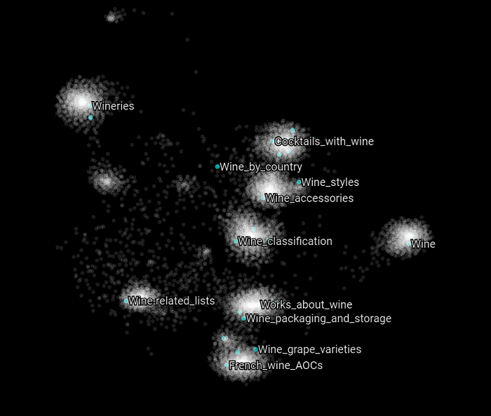
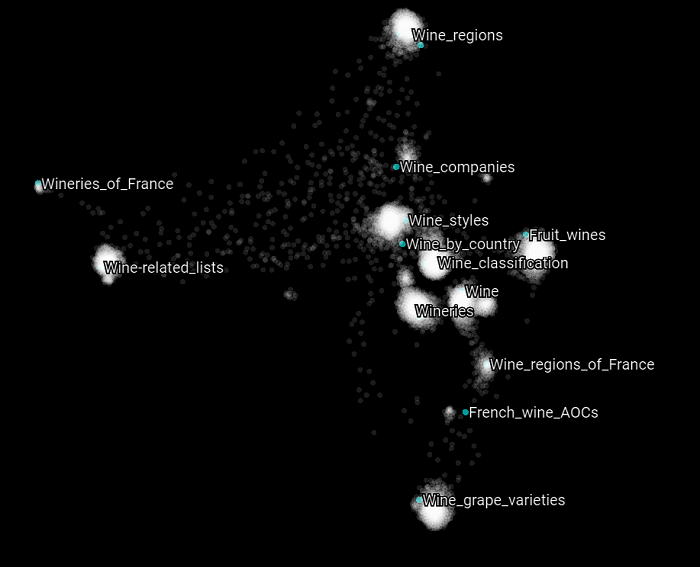
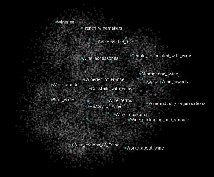
Here we highlight all the Wikipedia categories that have the word “wine” in them.
Experimenting With Multiple DeepWalk Hyperparameters
Now that we have optimized the SVM hyperparameters to find the best classification performences, let’s see how some of the hyperparameters related to the DeepWalk algorithm can influence the performance of the model. The DeepWalk algorithm’s hyperparameters we want to experiment with are:
- The number of dimensions of the graph embedding vectors (
:vector-size), and - The depth of the random walks (
walks-per-vertex).
Walk-length of Five
The first experiment we want to perform is to visualize how the DeepWalk algorithm reacts if we change the depth of the random walks from 15 steps to only 5. The first thing we have to do is to create the deep-walk object with a window-size of 15 and a vector-size of 3. Nothing else changes here in this experiment.
(def deep-walk (create-deep-walk graph
                                 :window-size 15
                                 :vector-size 3
                                 :learning-rate 0.025))
Then when we train the model, we want the algorithm to go five steps for each vertex in the graph instead of 15.
(train deep-walk graph 5 175)
Then we create the create a new set of training and validation sets to evaluate the model.
(def model-vectors (build-svm-model-vectors "resources/core-wikipedia-subclass-mapped--extended.csv"
                                            deep-walk
                                            index
                                            :base-uri "http://wikipedia.org/wiki/Category:"))
We create a new SVM classification model trained on the new graph embedding vectors that have been created by DeepWalk with a walk-length of 20.
(def libsvm-model (svm.core/train-model (->> (:training model-vectors)
                                             (map (fn [item]
                                                    [(if (= (:class item) 0)
                                                       -1
                                                       1)
                                                     (->> (:f item)
                                                          (map (fn [[k v]]
                                                                 {(inc k) v}))
                                                          (apply merge))]))
                                             concat)
                                        :eps 0.2
                                        :gamma 1
                                        :probability 0
                                        :shrinking 0
                                        :nu 0.1
                                        :kernel-type (:rbf svm.core/kernel-types)
                                        :svm-type (:one-class svm.core/svm-types)))
Finally we evaluate the new model. Note that we used the optimal SVM hyperparameter values that we found with the grid search above. The results are somewhat equivalent with the previous ones we experienced.
(evaluate-libsvm-model model-vectors libsvm-model)
True positive:  1723
false positive:  395
True negative:  48
False negative:  209

Precision:  0.8135033
Recall:  0.8918219
Accuracy:  0.7456842
F1:  0.8508642
(generate-tensorflow-projector-vectors-libsvm model-vectors
                                              libsvm-model
                                              "kbpedia-projector-vectors-libsvm-wl5.csv"
                                              "kbpedia-projector-metadata-libsvm-wl5.csv")
However what we want to do is to visualize the new scatter plot generated by this new DeepWalk model. The following models have been created using DeepWalk with a walk-length of 5, 175 iterations and embedding vectors with 3 dimensions. The visualization has been created using the t-SNE algorithm with a perplexity of 25, a learning rate of 10 and 8500 iterations.
To load the following scatter plots, download this package, to do http://projector.tensorflow.org/, then load the vectors and metadata files. Finally load the bookmark using the txt file from the package.
Here is the 3-dimensional rendering of the scatter plot.
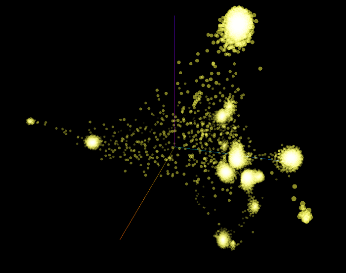
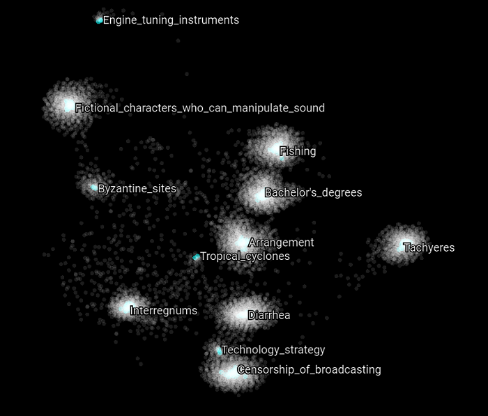
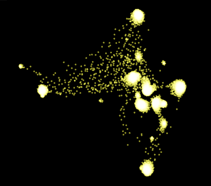
Here is the 2-dimensional rendering of the same graph composed of all the examples of the training and validation sets. If we compare this plot with the one that had a walk-length of 15, we can observe that most of the clusters are much closer to the other, which suggests that their distinctiveness is less pronounced than it was with a walk-length of 15. This intuitively make sense since we only walk 5 vertices of the graph instead of 15, then the upper structure of the Knowledge Graph has less impact on the over all structure (as exemplified by the graph embeddings) of each vertice.
Here we only focus on the negative examples of the validation set. We can see that each of the negative examples appears at the center of each cluster.
Here we only focus on the positive examples of the validation set.

Now let’s focus on specific Wikipedia categories that can belong to the training or the validation set. In the following scatter plot, we highlight all the categories that have the word “police” in them. What we can observe here compared to the previous version of this graph is that these Wikipedia categories appears closer to each other which suggest that the upper structure has less impact on how the over all categories are clustered (by their graph latent structure). Also, the Chiefs_of_police does not belong to any cluster, but it was when we used a walk-length of 15.
The same behavior can be observed for the categories that have “fire” in their name.
Finally exactly the same behavior can be observed for the categories that have “wine” in their name.
What we can conclude from changing the walk-length of the DeepWalk algorithm on such a Knowledge Graph is that it appears that it will have an impact on how the vertices will be represented and clustered by the t-SNE algorithm and how each other will be related one between the other considering their graph embeddings. A higher number for walk-length appears to be more beneficial, but takes more time to compute.
Nine Dimensions
Now let experiment when we increase the number of dimensions for the graph embeddings. Let’s increase the number of dimensions from three to nine. However let’s use the walk-length of 15. The first thing we have to do is to create the DeepWalk object with a :vector-size of nine.
(def deep-walk (create-deep-walk graph
                                 :window-size 15
                                 :vector-size 9
                                 :learning-rate 0.025))
Then we train the model with a walk-length of 15 and and 175 iterations.
(train deep-walk graph 15 175)
We re-create the training and validation sets to train the SVM classifier.
(def model-vectors (build-svm-model-vectors "resources/core-wikipedia-subclass-mapped--extended.csv"
                                            deep-walk
                                            index
                                            :base-uri "http://wikipedia.org/wiki/Category:"))
Then what we do is to re-run the grid search to find the optimal hyperparameters to properly configure the SVM classifier with these new graph embedding vectors as computed by the new DeepWalk model.
(svm-grid-search-one-class-rbf model-vectors :grid-parameters [{:gamma [1 1/2 1/3 1/4 1/5 1/7 1/10 1/50 1/100]
                                                                :eps [0.000001 0.00001 0.0001 0.001 0.01 0.1 0.2]
                                                                :nu [0.1 0.2 0.3 0.4 0.5 0.6 0.7 0.8 0.9]
                                                                :probability [0 1]
                                                                :shrinking [0 1]
                                                                :selection-metric :f1}])
(def libsvm-model-optimized (svm.core/train-model (->> (:training model-vectors)
                                                       (map (fn [item]
                                                              [(if (= (:class item) 0)
                                                                 -1
                                                                 1)
                                                               (->> (:f item)
                                                                    (map (fn [[k v]]
                                                                           {(inc k) v}))
                                                                    (apply merge))]))
                                                       concat)
                                                  :eps 0.1
                                                  :gamma 1
                                                  :nu 0.1
                                                  :probability 0
                                                  :shrinking 0
                                                  :kernel-type (:rbf svm.core/kernel-types)
                                                  :svm-type (:one-class svm.core/svm-types)))
(evaluate-libsvm-model model-vectors libsvm-model-optimized)
True positive:  1741
false positive:  422
True negative:  38
False negative:  174

Precision:  0.8049006
Recall:  0.9091384
Accuracy:  0.74905264
F1:  0.85384995
(generate-tensorflow-projector-vectors-libsvm model-vectors
                                              libsvm-model
                                              "kbpedia-projector-vectors-libsvm-wl15-d9.csv"
                                              "kbpedia-projector-metadata-libsvm-wl15-d9.csv")
Let’s visualize this new model that uses nine dimensions instead of three. The following models have been created using DeepWalk with a walk-length of 15, 175 iterations and embedding vectors with nine dimensions. The visualization has been created using the t-SNE algorithm with a perplexity of 25, a learning rate of 10 and 30,000 iterations.
To load the following scatter plots, download this package, to do http://projector.tensorflow.org/, then load the vectors and metadata files. Finally load the bookmark using the txt file from the package.
Now let’s visualize the graph of all the training and validation set examples reduced from nine dimensions to two. As you can see, this graph is quite different from the previous ones. We can see some kind of blurred clusters but everything is quite scattered.
The following graph highlight all the positive examples of the validation set.
Here are all the categories that belong to the negative examples of the validation set. There is no apparent structure for these two graphs. vertices just appear to be “randomly” displayed in the scatter plot.
Finally let’s highlight the Wikipedia categories that have the word “wine” in them.
What this experiment shows is how care should be taken when visualizing, and more importantly interpreting, these kind of visualization created by dimension reduction techniques such as PCA and t-SNE algorithms.
Classifying Candidates
Now that we have an adequate model in place, the last step of the process is to classify each of the candidates we previously found using the best optimized model we created so far. Remember that the goal is to find Wikipedia categories candidates that could create new KBpedia reference concepts which are not currently existing to extend the scope of the Knowledge Graph.
What we have to do is to iterate over all the candidates we found and to classify each of them according to their graph embedding vectors as classified by a SVM model configured using the best hyperparameters.
(defn classify-categories
  [svm-model possible-new-rc-csv classified-csv index deep-walk]
  (let [categories-csv (rest
                        (with-open [in-file (io/reader possible-new-rc-csv)]
                          (doall
                           (csv/read-csv in-file))))]
    (with-open [out-file (io/writer classified-csv)]
      (csv/write-csv out-file [["kbpedia-rc" "wikipedia-category" "possible-new-sub-class-of" "cognonto-classification"]])
      (doseq [[kbpedia-rc wikipedia-category possible-new-sub-class-of] categories-csv]
        (if (empty? possible-new-sub-class-of)
          (csv/write-csv out-file [[kbpedia-rc wikipedia-category possible-new-sub-class-of ""]])
          (csv/write-csv out-file [[kbpedia-rc wikipedia-category possible-new-sub-class-of
                                    (if (= (svm.core/predict svm-model
                                                             (into (sorted-map-by <)
                                                                   (->> (read-string
                                                                         (.toString
                                                                          (.data
                                                                           (.getVector
                                                                            (.lookupTable deep-walk)
                                                                            (get index (str "http://wikipedia.org/wiki/Category:" possible-new-sub-class-of))))))
                                                                        (map-indexed (fn [feature-id value]
                                                                                       {feature-id value}))
                                                                        (apply merge)))) 1.0)
                                      "x"
                                      "")]]))))))
(classify-categories libsvm-model-optimized "resources/leaf-rcs-narrower-concepts.csv" "resources/leaf-rcs-narrower-concepts--libsvm-classified.csv" index deep-walk)

(classify-categories libsvm-model-optimized "resources/near-leaf-rcs-narrower-concepts.csv" "resources/near-leaf-rcs-narrower-concepts--libsvm-classified.csv" index deep-walk)

(classify-categories libsvm-model-optimized "resources/core-wikipedia-subclass-mapped.csv" "resources/core-wikipedia-subclass-mapped--libsvm-classified.csv" index deep-walk)
The result of this classification task is that among all the candidates we identified, 20,653 have been classified to be possible new KBpedia reference concepts. These final candidates will then be reviewed by a KBpedia maintainer to make the final decision to determine if that concept should be added to KBpedia or not.
Conclusion
What we demonstrated in this article is how the inner structure of the KBpedia Knowledge Graph and its linkage to external conceptual structures such as the Wikipedia category structure can be leveraged to extend the scope of the Knowledge Graph.
Additionally we demonstrated how machine learning techniques such as DeepWalk and SVM classifiers can be used to filter potential candidates automatically to lower the time a human reviewer has to spend to take the final decision as to which new concepts will make it into the Knowledge Graph.
While the example herein is based on the Wikipedia category structure, any external schema or ontology may be handled in a similar way. The essential point is to create a system and workflow that enables huge numbers of combinatorial candidates to be winnowed down into likely candidates for manual approval. The systematic approach to the pipeline and the use of positive and negative training sets means that tuning the approach can be fully automated and rapidly vetted.
Many of these machine learning techniques are relatively new within the scientific literature. Applying them to these kind of tasks is novel to our knowledge. But more importantly, to our experience performing these tasks, the time spent by a human to extend such a big coherent and consistent Knowledge Graph can significantly be reduced by leveraging such techniques, which ultimately greatly reduces the development and maintenance costs of such Knowledge Graphs.
Footnotes:
1 Perozzi, B., Al-Rfou, R., & Skiena, S. (2014, August). Deepwalk: Online learning of social representations. In Proceedings of the 20th ACM SIGKDD international conference on Knowledge discovery and data mining (pp. 701-710). ACM.
2 Goodfellow, I., Bengio, Y. & Courville, A. (2016). Deep learning. Cambridge, MA: MIT Press.