A common task required by systems that automatically analyze text is to classify an input text into one or multiple classes. A model needs to be created to scope the class (what belongs to it and what does not) and then a classification algorithm uses this model to classify an input text.
Multiple classification algorithms exists to perform such a task: Support Vector Machine (SVM), K-Nearest Neigbours (KNN), C4.5 and others. What is hard with any such text classification task is not so much how to use these algorithms: they are generally easy to configure and use once implemented in a programming language. The hard – and time-consuming – part is to create a sound training corpus that will properly define the class you want to predict. Further, the steps required to create such a training corpus must be duplicated for each class you want to predict.
Since creating the training corpus is what is time consuming, this is where Cognonto provides its advantages.
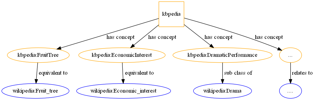
In this article, we will show you how Cognonto’s KBpedia Knowledge Graph can be used to automatically generate training corpuses that are used to generate classification models. First, we define (scope) a domain with one or multiple KBpedia reference concepts. Second, we aggregate the training corpus for that domain using the KBpedia Knowledge Graph and its linkages to external public datasets that are then used to populate the training corpus of the domain. Third, we use the Explicit Semantic Analysis (ESA) algorithm to create a vectorial representation of the training corpus. Fourth, we create a model using (in this use case) an SVM classifier. Finally, we predict if an input text belongs to the class (scoped domain) or not.
This use case can be used in any workflow that needs to pre-process any set of input texts where the objective is to classify relevant ones into a defined domain.
Unlike more traditional topic taggers where topics are tagged in an input text with weights provided for each of them, we will see how it is possible to use the semantic interpreter to tag main concepts related to an input text even if the surface form of the topic is not mentioned in the text. We accomplish this by leveraging ESA’s semantic interpreter.
[extoc]
General and Specific Domains
In this article, two concepts are at the center of everything: what I call the general domain and the specific domain(s). What I call the general domain can be seen as the set of all specific domains. It includes the set of classes that generally define common things of the World. What we call a specific domain is one or multiple classes that scope a domain of interest. A specific domain is a subset of classes of the general domain.
In Cognonto, the general domain is defined by all the ~39,000 KBpedia reference concepts. A specific domain is any sub-set of the ~39,000 KBpedia reference concept that adequately scopes a domain of interest.
The purpose of this use case is to show how we can determine if an input text belongs to a specific domain of interest. What we have to do is to create two training corpuses: one that defines the general domain, and one that defines the specific domain. However, how do we go about defining these corpuses? One way would be to do this manually, but it would take an awful lot of time to do.
This is the crux of the matter: we will generate the general domain corpus and specific domain ones automatically using the KBpedia Knowledge Graph and all of its linkages to external public datasets. The time and resources thus saved from creating the training corpuses can be spent testing different classification algorithms, tweaking their parameters, evaluating them, etc.
What is so powerful in leveraging the KBpedia Knowledge Graph in this manner is that we can generate training sets for all kind of domains of interests automatically.
Training Corpuses
The first step we have to do is to define the training corpuses that we will use to create the semantic interpreter and the SVM classification models. We have to create the general domain training corpus and the domain specific training corpus. The example domain I have chosen for this use case is scoped by the ideas of Music, Musicians, Music Records, Musical Groups, Musical Instruments, etc.
Define The General Training Corpus
The general training corpus is quite easy to create. The only thing I have to do is to query the KBpedia Knowledge Graph to get all the Wikipedia pages linked to all the KBpedia reference concepts. These pages will become the general training corpus.
Note that in this article I will only use the linkages to the Wikipedia dataset, but I could also use any other datasets that are linked to the KBpedia Knowledge Graph in exactly the same way. Here is how we aggregate all the documents that will belong to a training corpus:
Note all I need do is to use the KBpedia structure, query it, and then write the general corpus into a CSV file. This CSV file will be used later for most of the subsequent tasks.
(define-general-corpus "resources/kbpedia_reference_concepts_linkage.n3" "resources/general-corpus-dictionary.csv")
Define The Specific Domain Training Corpus
The next step is to define the training corpuse of the specific domain for this use case, the music domain. To do so, I need merely search KBpedia to find all the reference concepts I am interested in that will scope my music domain. These domain-specific KBpedia reference concepts will be the features of the SVM models we will test below.
What the define-domain-corpus function does below is simply to query KBpedia to get all the Wikipedia articles related to these concepts, their sub-classes and to create the training corpus from them.
In this article we only define a binary classifier. However, if we would want to create a multi-class classifier then we would have to define multiple specific domain training corpuses exactly the same way. The only time we would have to spend is to search KBpedia (using the Cognonto user interface) to find the reference concepts we want to use to scope the domains we want to define. We will show how quickly this can be done with impressive results in a later use case.
(define-domain-corpus ["http://kbpedia.org/kko/rc/Music"
                       "http://kbpedia.org/kko/rc/Musician"
                       "http://kbpedia.org/kko/rc/MusicPerformanceOrganization"
                       "http://kbpedia.org/kko/rc/MusicalInstrument"
                       "http://kbpedia.org/kko/rc/Album-CW"
                       "http://kbpedia.org/kko/rc/Album-IBO"
                       "http://kbpedia.org/kko/rc/MusicalComposition"
                       "http://kbpedia.org/kko/rc/MusicalText"
                       "http://kbpedia.org/kko/rc/PropositionalConceptualWork-MusicalGenre"
                       "http://kbpedia.org/kko/rc/MusicalPerformer"]
  "resources/kbpedia_reference_concepts_linkage.n3"
  "resources/domain-corpus-dictionary.csv")
Create Training Corpuses
Once the training corpuses are defined, we want to cache them locally to be able to play with them, without having to re-download them from the Web or re-create them each time.
(cache-corpus)
The cache is composed of 24,374 Wikipedia pages, which is about 2G of raw data. However, we have some more processing to perform on the raw Wikipedia pages since what we ultimately want is a set of relevant tokens (words) that will be used to calculate the value of the features of our model using the ESA semantic interpreter. Since we may want to experiment with different normalization rules, what we do is to re-write each document of the corpus in another folder that we will be able to re-create as required if the normalization rules change in the future. We can quickly re-process these input files and save them in separate folders for testing and comparative purposes.
The normalization steps performed by this function are to:
- Defluff the raw HTML page. We convert the HTML into text, and we only keep the body of the page
- Normalize the text with the following rules:
- remove diacritics characters
- remove everything between brackets like: [edit] [show]
- remove punctuation
- remove all numbers
- remove all invisible control characters
- remove all [math] symbols
- remove all words with 2 characters or fewer
- remove line and paragraph seperators
- remove anything that is not an alpha character
- normalize spaces
- put everything in lower case, and
- remove stop words.
Normalization steps could be dropped or others included, but these are the standard ones Cognonto applies in its baseline configuration.
(normalize-cached-corpus "resources/corpus/" "resources/corpus-normalized/")
After cleaning, the size of the cache is now 208M (instead of the initial 2G for the raw web pages).
Note that unlike what is discussed in the original ESA research papers by Evgeniy Gabrilovich we are not pruning any pages (the ones with less than X number of tokens, etc. This could be done but at a subsequent tweaking step, which our results below indicate is not really necessary.
Now that the training corpuses are created we can now build the semantic interpreter to create the vectors that will be used to train the SVM classifier.
Build Semantic Interpreter
What we want to do is to classify (determine) if an input text belongs to a class as defined by a domain. The relatedness of the input text is based on how closely the specific domain corpus is related to the general one. This classification is performed with some classifiers like SVM, KNN and C4.5. However, each of these algorithms need to use some kind of numerical vector, upon which the actual classifier requires to model and classify the candidate input text. Creating this numeric vector is the job of the ESA Semantic Interpreter.
Let’s dive a little further into the Semantic Interpreter to understand how it operates. Note that you can skip the next section and continue with the following one.
How Does the Semantic Interpreter Work?
The Semantic Interpreter is a process that maps fragments of natural language into a weighted sequence of text concepts ordered by their relevance to the input.
Each concept in the domain is accompanied by a document from the KBpedia Knowledge Graph, which acts as its representative term set to capture the idea (meaning) of the concept. The overall corpus is based on the combined documents from KBpedia that match the slice retrieved from the knowledge graph based on the domain query(ies).
The corpus is composed of ![]() concepts that come from the domain ontology associated with
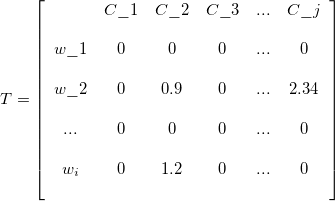
concepts that come from the domain ontology associated with ![]() KBpedia Knowledge Base documents. We build a sparse matrix
KBpedia Knowledge Base documents. We build a sparse matrix ![]() where each of the
where each of the ![]() columns corresponds to a concept and where each of the rows corresponds to a word that occurs in the related entity documents
columns corresponds to a concept and where each of the rows corresponds to a word that occurs in the related entity documents ![]() . The matrix entry
. The matrix entry ![]() is the TF-IDF value of the word
is the TF-IDF value of the word ![]() in document
in document ![]() .
.
The TF-IDF value of a given term is calculated as:
![]()
where ![]() is the number of words in the document
is the number of words in the document ![]() , where the term frequency is defined as:
, where the term frequency is defined as:
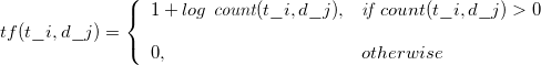
and where the document frequency ![]() is the number of documents where the term
is the number of documents where the term ![]() appears.
appears.
Unlike the standard ESA system, pruning is not performed on the matrix to remove the least-related concepts for any given word. We are not doing the pruning due to the fact that the ontologies are highly domain specific as opposed to really broad and general vocabularies. However, with a different mix of training text, and depending on the use case, the stardard ESA model may benefit from pruning the matrix.
Once the matrix is created, we do perform cosine normalization on each column:
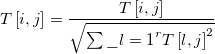
where ![]() is the TF-IDF weight of the word
is the TF-IDF weight of the word ![]() in the concept document
in the concept document ![]() , where
, where ![]() is the square root of the sum of exponent of the TF-IDF weight of each word
is the square root of the sum of exponent of the TF-IDF weight of each word ![]() in document
in document ![]() . This normalization removes, or at least lowers, the effect of the length of the input documents.
. This normalization removes, or at least lowers, the effect of the length of the input documents.
Creating the First Semantic Interpreter
The first semantic interpreter we will create is composed of the general corpus which has 24,374 Wikipedia pages and the music domain-specific corpus composed of 62 Wikipedia pages. The 62 Wikipedia pages that compose the music domain corpus come from the selected KBpedia reference concepts and their sub-classes that we defined in the Define The Specific Domain Training Corpus section above.
(load-dictionaries "resources/general-corpus-dictionary.csv" "resources/domain-corpus-dictionary--base.csv")

(build-semantic-interpreter "base" "resources/semantic-interpreters/base/" (distinct (concat (get-domain-pages) (get-general-pages))))
Evaluating Models
Before building the SVM classifier, we have to create a gold standard that we will use to evaluate the performance of the models we will test. What I did is to aggregate a list of news feeds from the CBC and from Reuters and then I crawled each of them to get the news they were containing. Once I aggregated each of them in a spreadsheet, I manually classified each of them. The result is a gold standard of 336 news pages which were classified as being related to the music domain or not. It can be downloaded from here.
Subsequently, three days later, I re-crawled the same feeds to create a second gold standard that has 345 new spages. It can be downloaded from here. I will use both to evaluate the different SVM models we will create below. (I created the two standards because of some internal tests and statistics we are compiling.)
Both gold standards got created this way:
(defn create-gold-standard-from-feeds
  [name]
  (let [feeds ["http://rss.cbc.ca/lineup/topstories.xml"
               "http://rss.cbc.ca/lineup/world.xml"
               "http://rss.cbc.ca/lineup/canada.xml"
               "http://rss.cbc.ca/lineup/politics.xml"
               "http://rss.cbc.ca/lineup/business.xml"
               "http://rss.cbc.ca/lineup/health.xml"
               "http://rss.cbc.ca/lineup/arts.xml"
               "http://rss.cbc.ca/lineup/technology.xml"
               "http://rss.cbc.ca/lineup/offbeat.xml"
               "http://www.cbc.ca/cmlink/rss-cbcaboriginal"
               "http://rss.cbc.ca/lineup/sports.xml"
               "http://rss.cbc.ca/lineup/canada-britishcolumbia.xml"
               "http://rss.cbc.ca/lineup/canada-calgary.xml"
               "http://rss.cbc.ca/lineup/canada-montreal.xml"
               "http://rss.cbc.ca/lineup/canada-pei.xml"
               "http://rss.cbc.ca/lineup/canada-ottawa.xml"
               "http://rss.cbc.ca/lineup/canada-toronto.xml"
               "http://rss.cbc.ca/lineup/canada-north.xml"
               "http://rss.cbc.ca/lineup/canada-manitoba.xml"
               "http://feeds.reuters.com/news/artsculture"
               "http://feeds.reuters.com/reuters/businessNews"
               "http://feeds.reuters.com/reuters/entertainment"
               "http://feeds.reuters.com/reuters/companyNews"
               "http://feeds.reuters.com/reuters/lifestyle"
               "http://feeds.reuters.com/reuters/healthNews"
               "http://feeds.reuters.com/reuters/MostRead"
               "http://feeds.reuters.com/reuters/peopleNews"
               "http://feeds.reuters.com/reuters/scienceNews"
               "http://feeds.reuters.com/reuters/technologyNews"
               "http://feeds.reuters.com/Reuters/domesticNews"
               "http://feeds.reuters.com/Reuters/worldNews"
               "http://feeds.reuters.com/reuters/USmediaDiversifiedNews"]]

    (with-open [out-file (io/writer (str "resources/" name ".csv"))]
      (csv/write-csv out-file [["class" "title" "url"]])
      (doseq [feed-url feeds]
        (doseq [item (:entries (feed/parse-feed feed-url))]
          (csv/write-csv out-file "" (:title item) (:link item) :append true))))))
Each of the different models we will test in the next sections will be evaluated using the following function:
(defn evaluate-model
  [evaluation-no gold-standard-file]
  (let [gold-standard (rest
                       (with-open [in-file (io/reader gold-standard-file)]
                         (doall
                          (csv/read-csv in-file))))
        true-positive (atom 0)
        false-positive (atom 0)
        true-negative (atom 0)
        false-negative (atom 0)]

    (with-open [out-file (io/writer (str "resources/evaluate-" evaluation-no ".csv"))]
      (csv/write-csv out-file [["class" "title" "url"]])

      (doseq [[class title url] gold-standard]
        (when-not (.exists (io/as-file (str "resources/gold-standard-cache/" (md5 url))))
          (spit (str "resources/gold-standard-cache/" (md5 url)) (slurp url)))
        (let [predicted-class (classify-text (-> (slurp (str "resources/gold-standard-cache/" (md5 url)))
                                                 defluff-content))]
          (println predicted-class " :: " title)
          (csv/write-csv out-file [[predicted-class title url]] :append true)
          (when (and (= class "1")
                     (= predicted-class 1.0))
            (swap! true-positive inc))

          (when (and (= class "0")
                     (= predicted-class 1.0))
            (swap! false-positive inc))

          (when (and (= class "0")
                     (= predicted-class 0.0))
            (swap! true-negative inc))

          (when (and (= class "1")
                     (= predicted-class 0.0))
            (swap! false-negative inc))))

      (println "True positive: " @true-positive)
      (println "false positive: " @false-positive)
      (println "True negative: " @true-negative)
      (println "False negative: " @false-negative)

      (println)

      (let [precision (float (/ @true-positive (+ @true-positive @false-positive)))
            recall (float (/ @true-positive (+ @true-positive @false-negative)))]
        (println "Precision: " precision)
        (println "Recall: " recall)
        (println "Accuracy: " (float (/ (+ @true-positive @true-negative) (+ @true-positive @false-negative @false-positive @true-negative))))
        (println "F1: " (float (* 2 (/ (* precision recall) (+ precision recall)))))))))
What this function does is to calculate the number of true-positive, false-positive, true-negative and false-negatives scores within the gold standard by applying the current model, and then to calculate the precision, recall, accuracy and F1 metrics. You can read more about how binary classifiers can be evaluated from here.
Build SVM Model
Now that we have numeric vector representations of the music domain and now that we have a way to evaluate the quality of the models we will be creating, we can now create and evaluate our prediction models.
The classification algorithm I choose to use for this article is the Support Vector Machine (SVM). I use the Java port of the LIBLINEAR library. Let’s create the first SVM model:
(build-svm-model-vectors "resources/svm/base/")
(train-svm-model "svm.w0" "resources/svm/base/"
                 :weights nil
                 :v nil
                 :c 1
                 :algorithm :l2l2)
This initial model is created using a training set that is composed of 24,311 documents that doesn’t belong to the class (the music specific domain), and 62 documents that does belong to that class.
Now, let’s evaluate how this initial model perform against the the two gold standards:
(evaluate-model "w0" "resources/gold-standard-1.csv" )
True positive:  5
False positive:  0
True negative:  310
False negative:  21

Precision:  1.0
Recall:  0.1923077
Accuracy:  0.9375
F1:  0.32258064
(evaluate-model "w0" "resources/gold-standard-2.csv" )
True positive:  2
false positive:  1
True negative:  319
False negative:  23

Precision:  0.6666667
Recall:  0.08
Accuracy:  0.93043476
F1:  0.14285713
Well, this first run looks like to be really poor! The issue here is a common issue with how the SVM classifier is being used. Ideally, the number of documents that belong to the class and the number of documents that do not belong to the class should be about the same. However, because of the way we defined the music specific domain, and because of the way we created the training corpuses, we ended up with two really unbalanced sets of training documents: 24,311 that doesn’t belong to the class and only 63 that does belong to the class. That is the reason why we are getting these kinds of poor results.
What can we do from here? We have two possibilities:
- We use LIBLINEAR’s weight modifier parameter to modify the weight of the terms that exists in the 63 documents that belong to the class. Because the two sets are so unbalanced, the weight should theorically be around 386, or
- We add thousands of new documents that belong to the class we want to predict.
Let’s test both options. We will initially play with the weights to see how much we can improve the current situation.
Improving Performance Using Weights
What we will do now is to create a series of models that will differ in the weight we will define to improve the weight of the classified terms in the SVM process.
Weight 10
(train-svm-model "svm.w10" "resources/svm/base/"
                 :weights {1 10.0}
                 :v nil
                 :c 1
                 :algorithm :l2l2)

(evaluate-model "w10" "resources/gold-standard-1.csv")
True positive:  17
False positive:  1
True negative:  309
False negative:  9

Precision:  0.9444444
Recall:  0.65384614
Accuracy:  0.9702381
F1:  0.77272725
(evaluate-model "w10" "resources/gold-standard-2.csv")
True positive:  15
False positive:  2
True negative:  318
False negative:  10

Precision:  0.88235295
Recall:  0.6
Accuracy:  0.9652174
F1:  0.71428573
This is already a clear improvement for both gold standards. Let’s see if we continue to see improvements if we continue to increase the weight.
Weight 25
(train-svm-model "svm.w25" "resources/svm/base/"
                 :weights {1 25.0}
                 :v nil
                 :c 1
                 :algorithm :l2l2)

(evaluate-model "w25" "resources/gold-standard-1.csv")
True positive:  20
False positive:  3
True negative:  307
False negative:  6

Precision:  0.8695652
Recall:  0.7692308
Accuracy:  0.97321427
F1:  0.8163265
(evaluate-model "w25" "resources/gold-standard-2.csv")
True positive:  21
False positive:  5
True negative:  315
False negative:  4

Precision:  0.8076923
Recall:  0.84
Accuracy:  0.973913
F1:  0.82352936
The general metrics continued to improve. By increasing the weight, the precision dropped a little bit, but the recall improved quite a bit. The overall F1 score significantly improved. Let’s see with the Weight at 50.
Weight 50
(train-svm-model "svm.w50" "resources/svm/base/"
                 :weights {1 50.0}
                 :v nil
                 :c 1
                 :algorithm :l2l2)

(evaluate-model "w50" "resources/gold-standard-1.csv")
True positive:  23
False positive:  7
True negative:  303
False negative:  3

Precision:  0.76666665
Recall:  0.88461536
Accuracy:  0.9702381
F1:  0.82142854
(evaluate-model "w50" "resources/gold-standard-2.csv")
True positive:  23
False positive:  6
True negative:  314
False negative:  2

Precision:  0.79310346
Recall:  0.92
Accuracy:  0.9768116
F1:  0.8518519
The trend continues: decline in precision increase of recall and overall F1 score is better in both cases. Let’s try with a weight of 200
Weight 200
(train-svm-model "svm.w200" "resources/svm/base/"
                 :weights {1 200.0}
                 :v nil
                 :c 1
                 :algorithm :l2l2)

(evaluate-model "w200" "resources/gold-standard-1.csv")
True positive:  23
False positive:  7
True negative:  303
False negative:  3

Precision:  0.76666665
Recall:  0.88461536
Accuracy:  0.9702381
F1:  0.82142854
(evaluate-model "w200" "resources/gold-standard-2.csv")
True positive:  23
False positive:  6
True negative:  314
False negative:  2

Precision:  0.79310346
Recall:  0.92
Accuracy:  0.9768116
F1:  0.8518519
Results are the same, it looks like improving the weights up to a certain point adds further to the predictive power. However, the goal of this article is not to be an SVM parametrization tutorial. Many other tests could be done such as testing different values for the different SVM parameters like the C parameter and others.
Improving Performance Using New Music Domain Documents
Now let’s see if we can improve the performance of the model even more by adding new documents that belong to the class we want to define in the SVM model. The idea of adding documents is good, but how may we quickly process thousands of new documents that belong to that class? Easy, we will use the KBpedia Knowledge Graph and its linkage to entities that exists into the KBpedia Knowledge Base to get thousands of new documents highly related to the music domain we are defining.
Here is how we will proceed. See how we use the type relationship between the classes and their individuals:

The millions of completely typed instances in KBpedia enable us to retrieve such large training sets efficiently and quickly.
Extending the Music Domain Model
To extend the music domain model I added about 5000 albums, musicians and bands documents using the relationships querying strategy outlined in the figure above. What I did is just to add 3 new features but with thousands of new training documents in the corpus.
What I had to do was to:
- Extend the domain pages with the new entities
- Cache the new entities’ Wikipedia pages
- Build a new semantic interpreter that take the new documents into account, and
- Build a new SVM model that use the new semantic interpreter’s output.
(extend-domain-pages-with-entities)
(cache-corpus)
(load-dictionaries "resources/general-corpus-dictionary.csv" "resources/domain-corpus-dictionary--extended.csv")

(build-semantic-interpreter "domain-extended" "resources/semantic-interpreters/domain-extended/" (distinct (concat (get-domain-pages) (get-general-pages))))

(build-svm-model-vectors "resources/svm/domain-extended/")
Evaluating the Extended Music Domain Model
Just like what we did for the first series of tests, we now will create different SVM models and evaluate them. Since we now have a nearly balanced set of training corpus documents, we will test much smaller weights (no weight, and then 2 weight).
(train-svm-model "svm.w0" "resources/svm/domain-extended/"
                 :weights nil
                 :v nil
                 :c 1
                 :algorithm :l2l2)

(evaluate-model "w0" "resources/gold-standard-1.csv")
True positive:  20
False positive:  12
True negative:  298
False negative:  6

Precision:  0.625
Recall:  0.7692308
Accuracy:  0.9464286
F1:  0.6896552
(evaluate-model "w0" "resources/gold-standard-2.csv")
True positive:  18
False positive:  17
True negative:  303
False negative:  7

Precision:  0.51428574
Recall:  0.72
Accuracy:  0.93043476
F1:  0.6
As we can see, the model is scoring much better than the previous one when the weight is zero. However, it is not as good as the previous one when weights are modified. Let’s see if we can benefit increasing the weight for this new training set:
(train-svm-model "svm.w2" "resources/svm/domain-extended/"
                 :weights {1 2.0}
                 :v nil
                 :c 1
                 :algorithm :l2l2)

(evaluate-model "w2" "resources/gold-standard-1.csv")
True positive:  21
False positive:  23
True negative:  287
False negative:  5

Precision:  0.47727272
Recall:  0.8076923
Accuracy:  0.9166667
F1:  0.59999996
(evaluate-model "w2" "resources/gold-standard-2.csv")
True positive:  20
False positive:  33
True negative:  287
False negative:  5

Precision:  0.3773585
Recall:  0.8
Accuracy:  0.8898551
F1:  0.51282054
Overall the models seems worse with weight 2, let’s try with weight 5:
(train-svm-model "svm.w5" "resources/svm/domain-extended/"
                 :weights {1 5.0}
                 :v nil
                 :c 1
                 :algorithm :l2l2)

(evaluate-model "w5" "resources/gold-standard-1.csv")
True positive:  25
False positive:  52
True negative:  258
False negative:  1

Precision:  0.32467532
Recall:  0.96153843
Accuracy:  0.8422619
F1:  0.4854369
(evaluate-model "w2" "resources/gold-standard-2.csv")
True positive:  23
False positive:  62
True negative:  258
False negative:  2

Precision:  0.27058825
Recall:  0.92
Accuracy:  0.81449276
F1:  0.41818184
The performances are just getting worse. But this makes sense at the same time. Now that the training set is balanced, there are many more tokens that participate into the semantic interpreter and so in the vectors generated by it and used by the SVM. If we increase the weight of a balanced training set, then this intuitively should re-unbalance the training set and worsen the performances. This is what is apparently happening.
Re-balancing the training set using this strategy does not look to be improving the prediction model, at least not for this domain and not for these SVM parameters.
Improving Using Manual Features Selection
So far, we have been able to test different kind of strategies to create different training corpuses, to select different features, etc. We have been able to do this within a day, mostly waiting for the desktop computer to build the semantic interpreter and the vectors for the training sets. It has been possible thanks to the KBpedia Knowledge Graph that enabled us to easily and automatically slice-and-dice the knowledge structure to perform all these tests quickly and efficiently.
There are other things we could do to continue to improve the prediction model, such as manually selecting features returned by KBpedia. Then we could test different parameters of the SVM classifier, etc. However, such tweaks are the possible topics of later use cases.
Multiclass Classification
Let me add a few additional words about multiclass classification. As we saw, we can easily define domains by selecting one or multiple KBpedia reference concepts and all of their sub-classes. This general process enables us to scope any domain we want to cover. Then we can use the KBpedia Knowledge Graph’s relationship with external data sources to create the training corpus for the scoped domain. Finally, we can use SVM as a binary classifier to determine if an input text belongs to the domain or not. However, what if we want to classify an input text with more than one domain?
This can easily be done by using the one-vs-rest (also called the one-vs-all) multiclass classification strategy. The only thing we have to do is to define multiple domains of interest, and then to create a SVM model for each of them. As noted above, this effort is almost solely one of posing one or more queries to KBpedia for a given domain. Finally, to predict if an input text belongs to any of each domain models we defined, we need to apply an SVM option (like LIBLINEAR) that already implements multi-class SVM classification.
Conclusion
In this article, we tested multiple, different strategies to create a good prediction model using SVM to classify input texts into a music-related class. We tested unbalanced training corpuses, balanced training corpuses, different set of features, etc. Some of these tests improved the prediction model; others made it worse. The key point that should be remembered is that any machine learning effort requires bounding, labeling, testing and refining multiple parameters in order to obtain the best results. Use of the KBpedia Knowledge Graph and its linkage to external public datasets enables Cognonto to now do this previously lengthy and time-consuming tasks quickly and efficiently.
Within a few hours, we created a classifier with an accuracy of about 97% that classifies input text to belong to a music domain or not. We demonstrate how we can create such classifiers more-or-less automatically using the KBpedia Knowledge Graph to define the scope of the domain and to classify new text into that domain based on relevant KBpedia reference concepts. Finally, we note how we may create multi-class classifiers using exactly the same mechanisms.