Graph Analysis of a Big Structure: UMBEL

In this blog post, I will show you how we can use basic graph analysis metrics to analyze Big Structures. I will do the analysis of the UMBEL reference concept structure to demonstration how graph and network analysis can be used to better understand the nature and organization of possible issues with Big Structures such as UMBEL.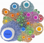

I will first present the formulas that have been used to perform the UMBEL analysis. To better understand this section, you will need some math knowledge, but there is nothing daunting here. You can probably safely skip that section if you desire.

The second section is the actual analysis of a Big Structure (UMBEL) using the graph measures I presented in the initial section. The results will be presented, analyzed and explained.

After reading this blog post, you should better understand how graph and network analysis techniques can be used to understand, use and leverage Big Structures to help integrate and interoperate disparate data sources.

[extoc]

Big Structure: Big in Size

A Big Structure is a network (a graph) of inter-related concepts which is composed of thousands or even hundred of thousands of such concepts. One characteristic of a Big Structure is its size. By nature, a Big Structure is too big to manipulate by hand and it requires tools and techniques to understand and assess the nature and the quality of the structure. It is for this reason that we have to leverage graph and network measures to help us in manipulating these Big Structures.

In the case of UMBEL, the Big Structure is a scaffolding of reference concepts used to link external (unrelated) structures to help data integration and to help unrelated systems inter-operate. In a World where the Internet Of Things is the focus of big companies and where there are more than 400 standards, such techniques and technologies are increasingly important, otherwise it will end-up being the Internet of [Individual] Things. Such a Big Structure can also be used for other tasks such as helping machine learning techniques to categorize and disambiguate pieces of data by leveraging such a structure of types.

UMBEL as a Graph

UMBEL is an RDF and OWL ontology of a bit more than 26 000 reference concepts. Because the structure is represented using RDF, it means that it is a directed graph. All of UMBEL’s vertices are classes, and all of the edges are properties.

The most important fact to keep in mind until the end of this blog post is that we are manipulating a directed graph. This means that all of the formulas used to analyze the UMBEL graph are formulas applicable to directed graphs only.

I will keep the normal graph analysis language that we use in the literature, however keep in mind that a vertice is a class or a named individual and that a edge is a property.

The UMBEL structure we are using is composed of the classes view and the individuals view of the ontology. That means that all the concepts are there, where some of them only have a class view, others have an individual view and others have both (because they got punned).

Graph Analysis Metrics

In this section, I will present the graph measures that we will use to perform the initial UMBEL graph analysis. In the next section, we will make the analysis of UMBEL using these measures, and we will discuss the results.

This section uses math notations. It could be skipped, but I suggest to try to take time some time to understand each measure since it will help to understand the analysis.

Some Notations

In this blog post, a graph is represented as $G = (V,E)$ where $G$ is the graph, $V$ is the set of all the vertices and $E$ is the set of all the edges of the same type that relates vertices.

The UMBEL analysis focuses on one of the following transitive properties:Â rdfs:subClassOf,Â umbel:superClassOf,Â skos:broaderTransitive, skos:narrowerTransitive and rdf:type. When we do perform the analysis, we are picking-up a subgraph that is composed of all the connections between the vertices that are linked by thisÂ edge (property).

Density

The first basic measure is the density of a graph. The density measures how many edges are in set $E$ compared to the maximum possible number of edges between vertices in set $V$ . The density is measured with:

$D = \frac{\raisebox{1.5mm}{$\vert E \vert$}}{\raisebox{-1.5mm}{$\vert V \vert ( \vert V \vert \mathbin{-} 1 )$}}$

where $D$ is the density, $E$ is the number of properties (edges) and $V$ is the number of classes (vertices).

The density is a ratio of the number of edges that exists, and the number of edges that could exists in the graph. $\vert E \vert$ is the number of edges in the graph and $\vert V \vert ( \vert V \vert \mathbin{-} 1 )$ is the number of possible maximum number of edges.

The maximum density is 1, and the minimum density is 0. The density of a graph gives us an idea about the number of connections that exists between the vertices.

Average Degree

The degree of a vertex is the number of edges that connect that vertex to other vertices. The average degree of a graph $G$ is another measure of how many edges are in set $E$ compared to number of vertices in set $V$ .

$\bar D = \frac{\raisebox{1.5mm}{$\vert E \vert$}}{\raisebox{-1.5mm}{$\vert V \vert$}}$

where $\bar D$ is the average degree, $E$ is the number of properties (edges) and $V$ is the number of classes (vertices).

This measure tells the average number of nodes to which any given node is connected.

Diameter

The diameter of a graph $G$ is the longest shortest path between two vertices in the graph. This means that this is the longest path that excludes all detours, loops, etc. between two vertices.

Let $d(v_{i},v_{j})$ be the length of the shortest path between $v_{i}$ and $v_{j}$ . And $v_{i}, v_{j} in V$ . The diameter of the graph is defined as:

$d = max(d(v_{i},v_{j}))$

This metric gives us an assessment of the size of the graph. It is useful to understand the kind of graph we are playing with. We will also relate it with the average path length to assess the span of the graph and the distribution of path lengths.

Average Path Length

The average path length is the average of the shortest path length, averaged over all pairs of vertices. Let $d(v_{i},v_{j})$ be the length of the shortest path between $v_{i}$ and $v_{j}$ . And $v_{i}, v_{j} in V$ .

$\bar P =\frac{\raisebox{1.5mm}{$ 1 $}}{\raisebox{-1.5mm}{$ N \cdot (N \mathbin{-} 1) $}} \cdot \sum_{i \neq j}^{} d(v_{i},v_{j})$

where, $N$ is the number of vertices in the graph $G$ ; where, $N \cdot (N \mathbin{-} 1)$ is the number of pairs of distinct vertices. Note that the number of pairs of distinct vertices is equal to the number of shortest paths between all pairs of vertices if we pick just one in case of a tie (two shortest paths with the same length).

In the context of ontology analysis, I would compare this metric as the speed of the ontology. What I mean by that is that one of the main tasks we do with an ontology is to infer new facts from known facts. Many inferring activities requires traversing the graph of an ontology. This means that the smaller the average path length between two classes, the more performant these inferencing activities should be.

Average Local Clustering Coefficient

The local clustering coefficient quantifies how well connected the neighborhood vertices of a given vertex are. It is the ratio of the edges that exists between all of the neighborhood vertices of a given vertex and the maximum number of possible edges between these same neighborhood vertices.

$C_{i} = \frac{\raisebox{1.5mm}{$\vert \lbrace e_{jk} : v_{j}, v_{k} \in N_{i}, e_{jk} \in E \rbrace \vert$}}{\raisebox{-1.5mm}{$k_{i} (k_{i} \mathbin{-} 1 $}}$

where $k_{i}$ is the number of neighborhood vertices, $$k_{i} (k_{i} \mathbin{-} 1 $})$ is the maximum number of edges between the neighborhood vertices and $\vert \lbrace e_{jk} : v_{j}, v_{k} \in N_{i}, e_{jk} \in E \rbrace \vert$ is the set of all the neighborhood vertices for a given vertex $e_{jk}$ .

The local clustering coefficient $\bar C$ is represented by the sum of the clustering coefficient of all the vertices of a graph $G$ divided by the number of vertices in $G$ . It is given by:

$\bar C = \sum_{i=1}^{n} \frac{C_{i}}{n}$

Betweenness Centrality

Betweenness centrality is a measure of importance of a node in a graph. It is represented by the number of times a node participates in the shortest path between other nodes. If a node participates in the shortest path of multiple other nodes, then it means that it is more important than other nodes in the graph. It acts like a conduit.

$g(v) = \sum_{s \neq v \neq t}^{} \frac{\raisebox{1.5mm}{$\sigma_{st}(v)$}}{\raisebox{-1.5mm}{$\sigma_{st}$}}$

where $\sigma_{st}$ is the total number of shortest paths from node $s$ to node $t$ and $\sigma_{st}(v)$ is the number of those paths that pass through $v$ .

In the context of ontology analysis, the betweenness centrality will tell us which of the classes that participates the more often in the shortest paths of a given transitive property between other classes. This measure is interesting to help us understand how a subgraph is constructed. For example, if we take a transitive property such as rdfs:subClassOf, then the graphs generated by a subgraph composed of this relationship only should be more hierarchic by the semantic nature of the property. This means that the nodes (classes) with the highest betweenness centrality value should be classes that participate in the upper portion of the ontology (the more general classes). However, if we think about the foaf:knows transitive property between named individuals, then the results should be quite different and suggest a different kind of graph.

Initial UMBEL Graph Analysis

Now that we have a good understanding of some core graph analysis measures, we will use them to analyze the graph of relationship between the UMBEL classes and reference concepts using the subgraphs generated by the properties: rdfs:subClassOf, umbel:superClassOf, skos:broaderTransitive, skos:narrowerTransitive and rdf:type.

Density

The maximum number of edges in UMBEL is: $26 345 * (26 345 - 1) = 694 032 680$ which is about two thirds of a billion of edges. This is quite a lot of edges, but it is important to keep in mind since most of the following ratios are based on this maximum number of edges (connections) between the nodes of the UMBEL graph.

Here is the table that shows the density of each subgraph generated by each property:

	Class view		Individual view
Metric	sub class of	super class of	broader	narrower	type
Number of edges	39 410	116 792	36 016	36 322	271 810
Density	0.0000567	0.0001402	0.0000518	0.0000523	0.0001021

As you can see, the density of any of the UMBEL subgraphs is really low considering that the maximum density of the graph is 1. However this gives us a picture of the structure: Most of the concepts have no more than few connections between each node for any of the analyzed properties.

This makes sense, since a conceptual structure is meant to model relationships between concepts that represent concepts of the real world, and in the real world, the concepts that we created are far from being connected to every other concept.

This is actually what we want: we want a conceptual structure which has a really low density. This suggest that the concepts are unambiguously related and hierarchized.

Having a high density (let’s say, 0.01, which would mean that there are nearly 7 million connections between the 26 345 concepts for a given property) may suggest that the concepts are too highly connected which could suggest that using the UMBEL ontology for tagging, classifying and reasoning over its concepts won’t be an optimal choice because of the nature of the structure and its connectivity (and possible lack of hierarchy).

Average Degree

The average degree shows the average number of UMBEL nodes that are connected to any other node for one of the given property.

	Class view		Individual view
Metric	sub class of	super class of	broader	narrower	type
Number of Edges	39406	97323	36016	36322	70921
Number of Vertices	26345	26345	26345	26345	26345
Average degree	1.4957	3.6941	1.3670	1.3787	2.6920

As you can see, the number are quite low: from 1.36 to 3.69. This is consistent with what we saw with the density measure above. This helps confirm our assumption that all of these properties create mostly hierarchical subgraphs.

However there seems to be one anomaly with these results, the average degree 3.69 of the umbel:superClassOf property. Intuitively, its degree should be near the one of the rdfs:subClassOf but it is far from this: it is more than twice its average degree. Looking at the OWL serialization of the UMBEL version 1.05 reveals that most umbel:RefConcept do have 3 triples:

  umbel:superClassOf skos:Collection ,
                     skos:ConceptScheme ,
                     skos:OrderedCollection .

This makes no sense that the umbel:RefConcept are super classes of these skos classes. I suspect that this got introduced via punning at some point in the history of UMBEL and got unnoticed until today. This issue will be fixed in a coming maintenance version of UMBEL.

If we check back the density measure of the graph, we notice that we have a density of 0.0001402 for the umbel:superClassOf property versus 0.0000567 for the rdfs:subClassOf property which has about the same ratio. So we could have noticed the same anomaly by taking a better look at the density measure.

But in any case, this shows how this kind of graph analysis can be used to find such issues in Big Structures (structures too big to find all these issues by scrolling the code only).

Diameter

The diameter of the UMBEL graph is like the worse case scenario. It tells us what is the longest shortest path for a given property’s subgraph.

	Class view		Individual view
Metric	sub class of	super class of	broader	narrower	type
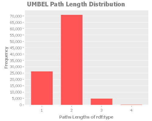
Diameter	19	19	19	19	4

In this case, this tell us that the longest shortest path between two given nodes for the rdfs:subClassOf property is 19. So in the worse case, if we infer something between these two nodes, then our algorithms will require maximum 19 steps (think in terms of a breath first search, etc).

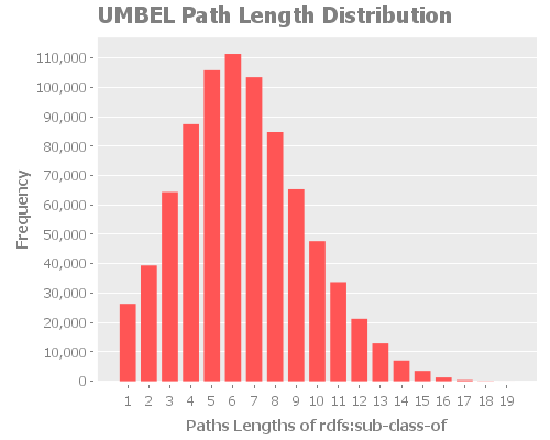
Average Path Length Distribution

The average path length distribution shows us the a number paths that have x in length. Because of the nature of UMBEL and its relationships, I think we should expect a normal distribution. An interesting observation we can do is the the average path length is situated around 6, which is the six degree of separation.

We saw that the “worse case scenario” was a shortest path of 19 for all the property except rdf:type. Now we know that the average is around 6.

rdfs:SubClassOf

umbel:superClassOf

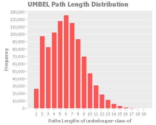
Here we can notice an anomaly in the expected normal distribution of the path lengths. Considering the other analysis we did, we can consider that the anomaly is related to the umbel:superClassOf issue we found. What we will have to re-check this metric once we fix the issue. I expect we will see a return to a normal distribution.

skos:broaderTransitive

skos:narrowerTransitive

rdf:type

Average Local Clustering Coefficient

The average local clustering coefficient will tell us how clustered the UMBEL subgraphs are.

	Class view		Individual view
Metric	sub class of	super class of	broader	narrower	type
Average local clustering coefficient	0.0001201	0.00000388	0.03004554	0.00094251	0.77191429

As we can notice, UMBEL does not have the small-world effect with its small clustering coefficients depending on the properties we are looking at. It means that there is not a big number of hubs in the network and so that the number of steps from going from a class or a reference concept to another is higher than in other kinds of networks, like airport networks. This makes sense by looking at the average path length and the path length distributions we observed above.

At the same time, this is the nature of the UMBEL graph: it is meant to be a a well structured set of concepts with multiple different specificity layers.

To understand its nature, we could consider the robustness of the network. Normally, networks with high average clustering coefficients are known to be robust, which means that if a random node is removed, it shouldn’t impact the average clustering coefficient or the average path length of that network. However, in a network that doesn’t have the small-world effect, then they are considered less robust which means that if a node is removed, it could greatly impact the clustering coefficients (which would be lower) and the average path length (which would be higher).

This makes sense in such a conceptual network: if we remove a concept from the structure, it will most than likely impact the connectivity of the other concepts of the network.

One interesting thing to notice is the clustering coefficient of 0.03 for the skos:broaderTransitive property and 0.00012 for the rdfs:subClassOf property. I have no explanation for this discrepancy at the moment, but this should be investigated after the fix as well since intuitively these two coefficient should be close.

Betweenness Centrality

As I said above, In the context of ontology analysis, the betweenness centrality tells us which of the classes participates more often in the shortest paths of a given transitive property between other classes. This measure is useful to help us understand how a subgraph is constructed.

If we check the results below, we can see that all the top nodes are nodes that we could easily classify as being part of the upper portion of the UMBEL ontology (the general concepts). Another interesting thing to notice is that the issue we found with the umbel:superClassOf property doesn’t seem to have any impact on the betweenness centrality of this subgraph.

rdfs:subClassOf

PartiallyTangible	0.1853398395065167
HomoSapiens	0.1184076250864128
EnduringThing_Localized	0.1081317879905902
SpatialThing_Localized	0.092787668995485
HomoGenus	0.07956810084399618

You can download the full list from here

umbel:superClassOf

PartiallyTangible	0.1538140444614064
HomoSapiens	0.1053345447606491
EnduringThing_Localized	0.08982813055659158
SuperType	0.08545549956197795
Animal	0.06988077993945754

You can download the full list from here

skos:broaderTransitive

PartiallyTangible	0.2051286996513612
EnduringThing_Localized	0.1298479341295156
HomoSapiens	0.09859060900526667
Person	0.09607892589570508
HomoGenus	0.08806468362881092

You can download the full list from here

skos:narrowerTransitive

PartiallyTangible	0.2064665713447941
EnduringThing_Localized	0.1294085106511612
HomoSapiens	0.1019893654646639
Person	0.09366129700219764
HomoGenus	0.09047063411213117

You can download the full list from here

rdf:type

owl:Class	0.3452564052004049
RefConcept	0.3424169525837704
ExistingObjectType	0.0856962574437039
ObjectType	0.01990245954437302
TemporalStuffType	0.01716817183946576

You can download the full list from here

Analysis with Inferred UMBEL

Now, let’s push the analysis further. Remember that I mentioned that all the properties we are analyzing in this blog post are transitive? Let’s perform exactly the same metrics analysis, but this time we will use the transitive closure of the subgraphs.

The transitivity characteristic of a property is simple to understand. Let’s consider this tiny graph $A \xrightarrow{p^{t}} B \xrightarrow{p^{t}} C$ where the property $\xrightarrow{p^{t}}$ is a transitive property. Since $\xrightarrow{p^{t}}$ is transitive, there is also a relationship $A \xrightarrow{p^{t}} C$ .

Given $A \xrightarrow{p^{t}} B \xrightarrow{p^{t}} C$ we inferred $A \xrightarrow{p^{t}} C$ using the transitive relation $\xrightarrow{p^{t}}$ .

Now, let’s use the power of these transitive properties and let’s analyze the transitive closure of the subgraphs that we are using to compute the metrics. The transitive closure is simple to understand. From the input subgraph, we are generating a new graph where all these transitive relations are explicit.

Let’s illustrate that using this small graph: $A \xrightarrow{p^{t}} B \xrightarrow{p^{t}} C, B \xrightarrow{p^{t}} D$ . The transitive clojure would create a new graph: $A \xrightarrow{p^{t}} B \xrightarrow{p^{t}} C, B \xrightarrow{p^{t}} D, A \xrightarrow{p^{t}} C, A \xrightarrow{p^{t}} D$

This is exactly what we will be doing with the sub-graphs created by the properties we are analyzing in this blog post. The end result is that we will be analyzing a graph with many more edges than we previously had with the non transitive closure versions of the subgraphs.

What we will analyze now is the impact of considering the transitive closure upon the ontology metrics analysis.

Density

Remember that the maximum number of edges in UMBEL is: $26 345 * (26 345 - 1) = 694 032 680$ , which is about two thirds of a billion edges.

	Class view		Individual view
Metric	sub class of	super class of	broader	narrower	type
Number of Edges	789 814	922 328	674 061	661 629	76 074
Density	0.0011380	0.0013289	0.0009712	0.0009533	0.0001096

As we can see, we have many more edges now with the transitive closure. The density of the graph is higher as well since we inferred new relationships between nodes from the transitive nature of the properties. However it is still low considering the number of possible edges between all nodes of the UMBEL graph.

Average Degree

We now see the impact of transitive closure on the average degree of the subgraphs. Now each node of the subgraphs are connected by 25 to 35 other nodes in average.

	Class view		Individual view
Metric	sub class of	super class of	broader	narrower	type
Number of Edges	789 814	922 328	674 061	661 629	76 074
Number of Vertices	26345	26345	26345	26345	26345
Average degree	29.97965	35.00960	25.58591	25.11402	2.887606

One interesting fact is that the anomaly disappears with this transitive closure subgraph for the umbel:superClassOf property. There is still a glitch with it, but I don’t think it would raise suspicion at first. This is important to note since we won’t have noticed this issue with the current version of the UMBEL ontology if we would have analyzed the transitive closure of the subgraph only.

Diameter

	Class view		Individual view
Metric	sub class of	super class of	broader	narrower	type
Diameter	2	2	2	2	2

As expected, the diameter of any of the transitive closure subgraphs is 2. It is the case since we made explicit a fact (a edge) between two nodes that was not explicit at first. This is good, but this is no quite useful from the perspective of ontology analysis.

This would only be helpful if the number were not 2 which would suggest some errors in the way you computed the diameter of the graph.

However what we can see here is that the speed of the ontology (as defined in the Average Path Length section above) is greatly improved. Since we forward-chained the facts in the transitive closure sub-graphs, it means that knowing if a class A is a sub-class of a class B is much faster, since we have a single lookup to do instead of an average of 6 for the non transitive closure version of the subgraphs.

Average Path Length Distribution

All of the path length distributions will be the same as this one:

Since the diameter is 2, then we have a full lot of paths at 2, and 26 345 at 1. This is not really that helpful from the standpoint of ontology analysis.

Average Local Clustering Coefficient

	Class view		Individual view
Metric	sub class of	super class of	broader	narrower	type
Average local clustering coefficient	0.3281777	0.0604906	0.2704963	0.0138592	0.7590267

Some of the properties like the rdfs:subClassOf property shows a much stronger coefficient than with the non-transitive closure version. This is normal since all the nodes are connected to the other nodes down the paths. So, if a node in between disappears, then it won’t affect the connectivity of the subgraph since all the linkage that got inferred still remains.

This analysis also suggests that the transitive closure version of the subgraphs are much stronger (which makes sense too).

However I don’t think this metric is that important of a characteristic to check when we analyze reference ontologies since they do not need to be robust. They are not airport or telephonic networks that need to cope with disappearing nodes in the network.

Betweenness Centrality

What the betweenness centrality measure does with the transitive closure of the subgraphs is that it highlight the real top concepts of the ontology like Thing, Class, Individual, etc. Like most of the other measures, it blurs the details of the structure (which is not necessarily a good thing).

rdfs:subClassOf

SuperType	0.03317996389023238
AbstractLevel	0.02810408526564482
Thing	0.02772171675862925
Individual	0.02747482318621853
TopicsCategories	0.02638342698407473

You can download the full list from here

umbel:superClassOf

The interesting thing here is that this measure actual shows the actual concepts for which we discovered an issue with above.

skos:Concept	0.02849203320293865
owl:Thing	0.02849094898994718
SuperType	0.02848878056396423
skos:ConceptScheme	0.02825567477079737
skos:OrderedCollection	0.02825567477079737

You can download the full list from here

skos:broaderTransitive

Thing	0.03225428380683926
Individual	0.03196350419108375
Location_Underspecified	0.0261924189600178
Region_Underspecified	0.02618796825161338
TemporalThing	0.02594169571990208

You can download the full list from here

skos:narrowerTransitive

Thing	0.03298126713602109
Location_Underspecified	0.02680852092899528
Region_Underspecified	0.02680398659044947
TemporalThing	0.02648809433842489
SomethingExisting	0.02582305801837314

You can download the full list from here

rdf:type

owl:Class	0.3452564052004049
RefConcept	0.342338078899975
ExistingObjectType	0.0856962574437039
ObjectType	0.01990245954437302
TemporalStuffType	0.01716817183946576

You can download the full list from here

Conclusion

This blog post shows that simple graph analysis metrics applied to Big Structures can be quite helpful to understand their nature, how they have been constructed, what is their size, their impact on some algorithms that could use them, and to find potential issues in the structure.

One thing we found is that the correlation between the properties rdfs:subClassOf and skos:broaderTransitive are nearly identical. They nearly have the same values for each metrics. If you were new to the UMBEL ontology you wouldn’t have known this fact without doing this kind of analysis or by spending much time looking at the serialized OWL file. It doesn’t tell us anything about how similar the relations are, but it does tell us that they have the same impact on the ontology’s graph structure.

Performing this analysis also led us to discover a few anomalies with the umbel:superClassOf property, suggesting an issue with the current version of the ontology. This issue would have been hard to notice, and understand, without performing such a graph analysis to the structure.

However, I also had the intuition that the analysis of the transitive closure of the subgraphs would have led to more interesting results. At best that analysis did confirm a few things, but in most of the cases it only blurred the specificities of most of the metrics.

These analysis metrics will soon be made available as standard Web services, so that they may be applied against any arbitrary graph or ontology.

3 thoughts on “Graph Analysis of a Big Structure: UMBEL”

Mark Martens

August 13, 2014 — 1:20 pm

Frederick, Good stuff, and a fascinating set of applications in my head.

Frederick Giasson

August 13, 2014 — 1:32 pm

Hi Mark,

Thanks for your comment. Don’t hesitate to shares what you have in mind in this comment section. It is all about understanding and using Big Structures for data integration and inter-operability in different contexts (from more traditional data integration task to more sophisticated AI development)

Thanks,

Fred

The Viking Algorithm for Connected Networks | AI3:::Adaptive Information

Big Structure: Big in Size

UMBEL as a Graph

Graph Analysis Metrics

Some Notations

Density

Average Degree

Diameter

Average Path Length

Average Local Clustering Coefficient

Betweenness Centrality

Initial UMBEL Graph Analysis

Density

Average Degree

Diameter

Average Path Length Distribution

rdfs:SubClassOf

umbel:superClassOf

skos:broaderTransitive

skos:narrowerTransitive

rdf:type

Average Local Clustering Coefficient

Betweenness Centrality

rdfs:subClassOf

umbel:superClassOf

skos:broaderTransitive

skos:narrowerTransitive

rdf:type

Analysis with Inferred UMBEL

Density

Average Degree

Diameter

Average Path Length Distribution

Average Local Clustering Coefficient

Betweenness Centrality

rdfs:subClassOf

umbel:superClassOf

skos:broaderTransitive

skos:narrowerTransitive

rdf:type

Conclusion

3 thoughts on “Graph Analysis of a Big Structure: UMBEL”

Mark Martens

Frederick Giasson

Leave a Reply Cancel reply