In a previous blog post, I explained how we can easily deploy Hugging Face models in Docker containers. In this new post, I will explain how we can easily deploy that container in Azure using Terraform. At the end of this article, we will have end-to-end process that creates a translation service, containerize, deploy in the cloud and that is readily available on the Web in a single command in your terminal.
Create Free Azure Account
If you don’t currently have access to an Azure account, you can easily create one for free here. You get a series of popular services for free for 12 months, 55 services free forever and 200$ USD in credit for a month. This is more than enough to run the commands in this tutorial. Even if none of those benefits would exists, it won’t be that much of a problem since you could create and tears down the services within a minute with terraform destroy which would incurs a few cents of usage.
Finally, make sure that you install the Azure CLI command line tool.
Install Terraform
The next step is to install Terraform on your local computer.
Terraform is an infrastructure-as-code (IaC) tool that allows users to define and manage their cloud infrastructure in a declarative manner (i.e. the infrastructure that is described in a Terraform file is the end-state of that infrastructure in the Cloud). It automates the process of provisioning and managing resources across various cloud providers, enabling consistent and reproducible deployments.
Using Terraform
This blog post is not meant to be an introduction to Terraform, so I will only cover the key commands that I will be using. There are excellent documentation by HashiCorp for developers and there are excellent books such as Terraform: Up and Running: Writing Infrastructure as Code by Yevgeniy Brikman.
The commands we will be using in this post are:
-
terraform plan: It is used to preview the changes that Terraform will make to the infrastructure. It analyzes the configuration files and compares the desired state with the current state of the resources. It provides a detailed report of what will be added, modified, or deleted. It does not make any actual changes to the infrastructure. -
terraform apply: It is used to apply the changes defined in the Terraform configuration files to the actual infrastructure. It will do the same asterraform plan, but at the end of the process it will prompt for confirmation before making any modifications. When we sayyes, then all hells are breaking loose in the Cloud and the changes are applied by Terraform. -
terraform destroy: It is used to destroy all the resources created and managed by Terraform. It effectively removes the infrastructure defined in the configuration files. It prompts for confirmation before executing the destruction.
Terraform file to deploy Hugging Face models on Azure
Now, let’s analyze the terraform file that tells Terraform how to create the infrastructure required to run the translation service in the Cloud.
Terraform Block
This terraform block is used to define the specific versions of Terraform and its providers. This ensure the reproducibility of the service over time, just like all the set versions of the libraries used for the translation service in Python.
terraform {
  required_version = ">= 1.5.6"

  required_providers {
    azurerm = {
      source  = "hashicorp/azurerm"
      version = ">= 3.71.0"
    }
    null = {
      source  = "hashicorp/null"
      version = ">= 3.2.1"
    }
  }
}
AzureRM Provider Block
This block configures the AzureRM provider. The skip_provider_registration prevents the provider from attempting automatic registration. The features {} specifies that no additional features for the provider are required for this demo.
provider "azurerm" {
  skip_provider_registration = "true"
  features {}
}
Resource Group Block
This block creates an Azure Resource Group (ARG) named translationarg in the eastus region. The resource group is what is used to bundle all the other resources we will require for the translation service.
resource "azurerm_resource_group" "acr" {
  name     = "translationarg"
  location = "eastus"
}
Container Registry Block
This block creates an Azure Container Registry (ACR) named translationacr. It associates the ACR with the previously defined resource group, in the same region. The ACR is set to the “Standard” SKU. admin_enabled allows admin access to the registry.
resource "azurerm_container_registry" "acr" {
  name                     = "translationacr"
  resource_group_name      = azurerm_resource_group.acr.name
  location                 = azurerm_resource_group.acr.location
  sku                      = "Standard"
  admin_enabled            = true
}
Null Resource for Building and Pushing Docker Image
This block uses the Null Provider and defines a null_resource used for building and pushing the Docker image where the translation service is deployed. It has a dependence on the creation of the Azure Container Registry, which means that the ACR needs to be created before this resource. The triggers section is set to a timestamp, ensuring the Docker build is triggered on every Terraform apply. The local-exec provisioner runs the specified shell commands for building, tagging, and pushing the Docker image.
resource "null_resource" "build_and_push_image" {
depends_on = [azurerm_container_registry.acr]
triggers = {
# Add a trigger to detect changes in your Docker build context
# The timestamp forces Terraform to trigger the Docker build,
# every time terraform is applied. The check to see if anything
# needs to be updated in the Docker container is delegated
# to Docker.
build_trigger = timestamp()
}
provisioner "local-exec" {
# Replace with the commands to build and push your Docker image to the ACR
command = <<EOT
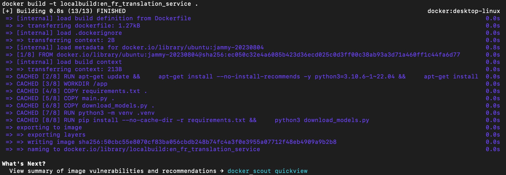
# Build the Docker image
docker build -t en-fr-translation-service:v1 ../../
# Log in to the ACR
az acr login --name translationacr
# Tag the Docker image for ACR
docker tag en-fr-translation-service:v1 translationacr.azurecr.io/en-fr-translation-service:v1
# Push the Docker image to ACR
docker push translationacr.azurecr.io/en-fr-translation-service:v1
EOT
}
}Container Group Block
This block creates an Azure Container Group (ACG). This is the resource used to create a container instance from a Docker container. It depends on the null_resource above for creating the image of the container and to make it available to the ACG.
The lifecycle block ensures that this container group is replaced when the Docker image is updated. Various properties like name, location, resource group, IP address type, DNS label, and operating system are specified. The image_registry_credential section provides authentication details for the Azure Container Registry. A container is defined with its name, image, CPU, memory, and port settings. Those CPU and Memory are required for the service with the current model that is embedded in the Docker container. Lowering those values may result in the container instance to die silently with a out of memory error.
resource "azurerm_container_group" "acr" {
  depends_on = [null_resource.build_and_push_image]

  lifecycle {
    replace_triggered_by = [
      # Replace `azurerm_container_group` each time this instance of
      # the the Docker image is replaced.
      null_resource.build_and_push_image.id
    ]
  }

  name                = "translation-container-instance"
  location            = azurerm_resource_group.acr.location
  resource_group_name = azurerm_resource_group.acr.name
  ip_address_type     = "Public"
  dns_name_label      = "en-fr-translation-service"
  restart_policy      = "Never"
  os_type             = "Linux"

  image_registry_credential {
     username = azurerm_container_registry.acr.admin_username
     password = azurerm_container_registry.acr.admin_password
    server   = "translationacr.azurecr.io"
  }

  container {
    name   = "en-fr-translation-service-container"
    image  = "translationacr.azurecr.io/en-fr-translation-service:v1"
    cpu    = 4
    memory = 8

    ports {
      protocol = "TCP"
      port     = 6000
    }
  }

  tags = {
    environment = "development"
  }
}
Deploying the English/French Translation Service on Azure
Now that we have a Terraform file that does all the work for us, how can we deploy the service on Azure?
As simply as running this command line from the /terraform/deploy/ folder:
terraform applyOnce we run that command, Terraform will analyze the file, and show everything that will changes in the Cloud infrastructure. In this case, we start from scratch, so all those resources will be created (none will change nor be destroyed):
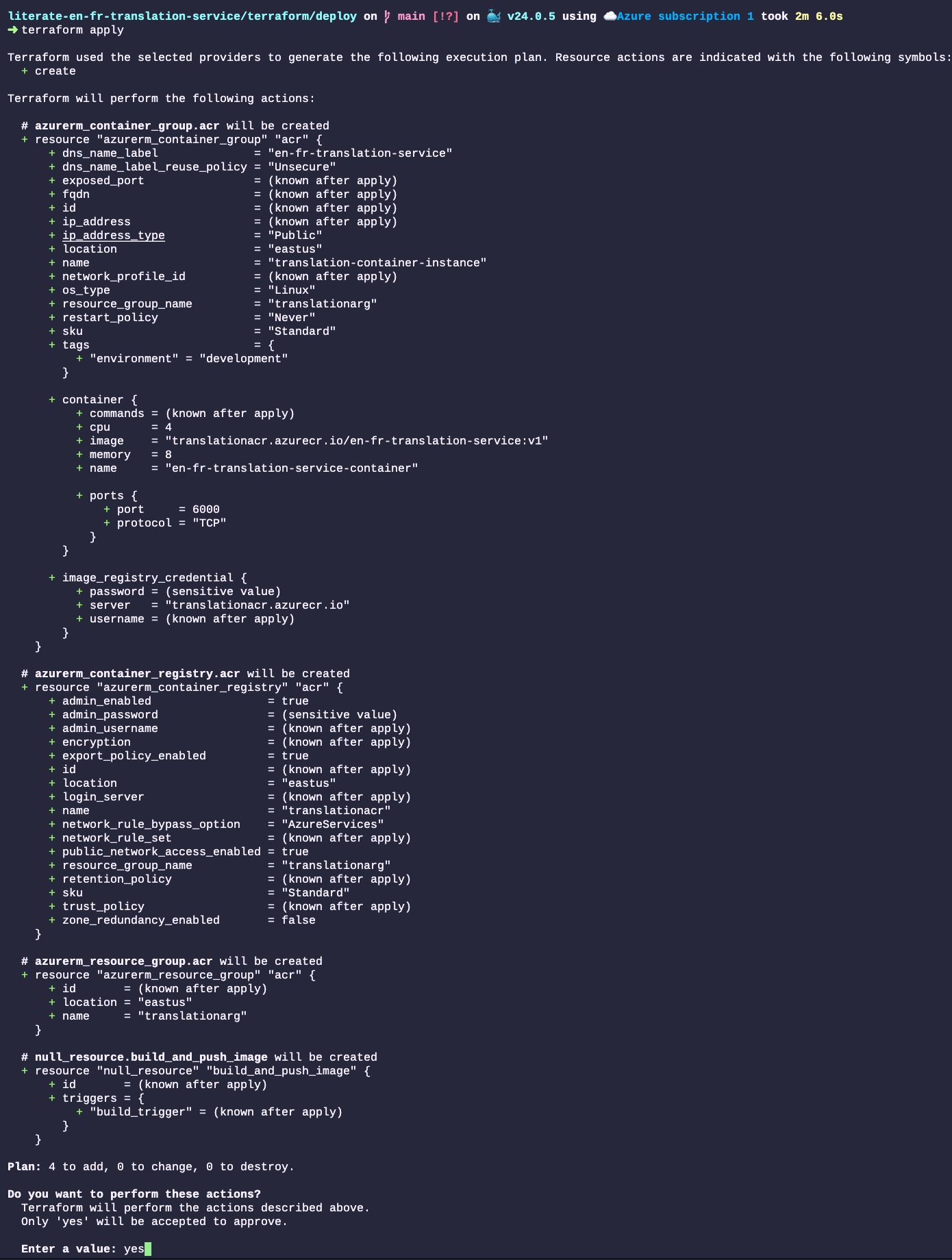
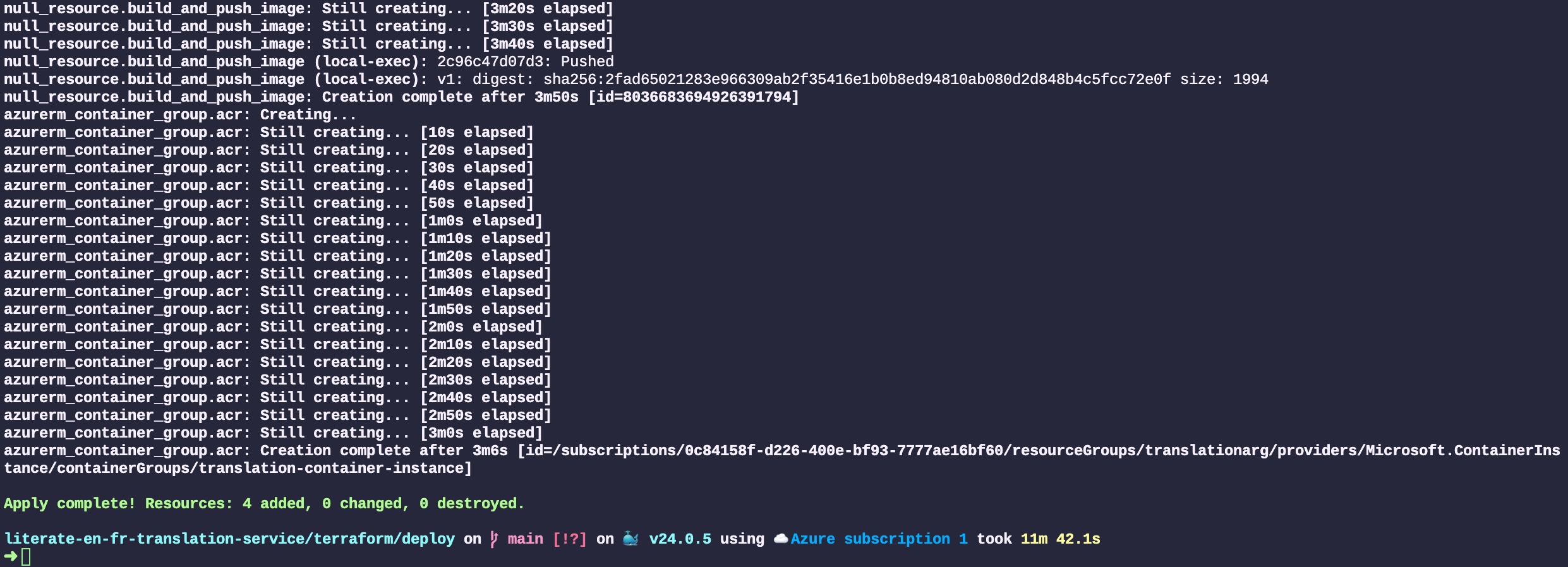
All the resources will then be created by Terraform. Those resources are created by communicating with Azure’s web service API. The output of each step is displayed in the terminal. The entire process to deploy four resources took about 12 minutes, 4 of which is to create the Docker image and 3 to create the Cloud resources and deploy the service. Most of the time is spent dealing with the somewhat big translation models that we baked in the Docker image:
Testing the Translation Service on Azure
The next step is to test the service we just created on Azure.
curl "http://en-fr-translation-service.eastus.azurecontainer.io:6000/translate/fr/en/" -H "Content-Type: application/json" -d '{"fr_text":"Bonjour le monde!"}'The result we get from the service:
{
  "en_text": "Hello, world!"
}
It works! (well, why would I have spent the time to write this post if it didn’t?)
A single command in your terminal to:
- Package a translation service and powerful translation models into a container image
- Creating a complete cloud infrastructure to support the service
- Deploy the image on the infrastructure and start the service
If this is not like magic, I wonder what that is.
Destroying Cloud Infrastructure
The last step is to destroy the entire infrastructure such that we don’t incur costs for those tests. The only thing that is required is to run the following Terraform command:
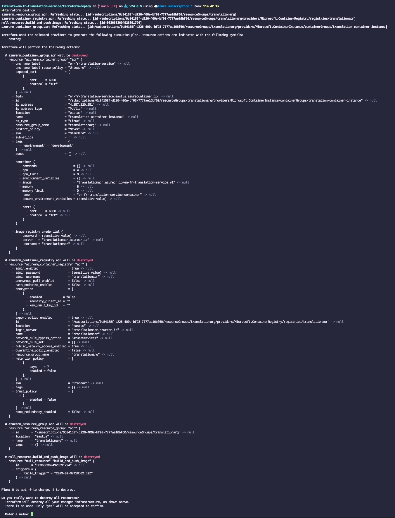
terraform destroyJust like with terraform apply, Terraform will check the current state of the cloud infrastructure (which is defined in the terraform.tfstate JSON file), will show all the resources that will be destroyed, and ask the user to confirm that they want to proceed by answering yes:
Linter
I would recommend that you always run your Terraform through a linter. There are several of them existing, none of them are mutually exclusive. Three popular ones are tflint, Checkov and Trivy. Checkov and Trivy are more focused on security risks.
For this blog post, I will only focus on tflint. Once you installed it, you can run it easily from your terminal:
tflintIf I run that command from the /terraform/deploy/ folder, and if I remove the Terraform version from the Terraform block, tflint will return the following error:
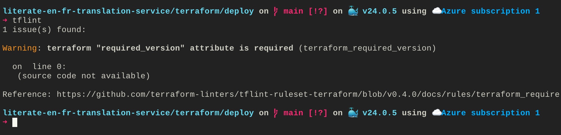
You can then follow the link to the Github documentation to understand what the error means and how to fix it.
Run Linter every time you update your repository
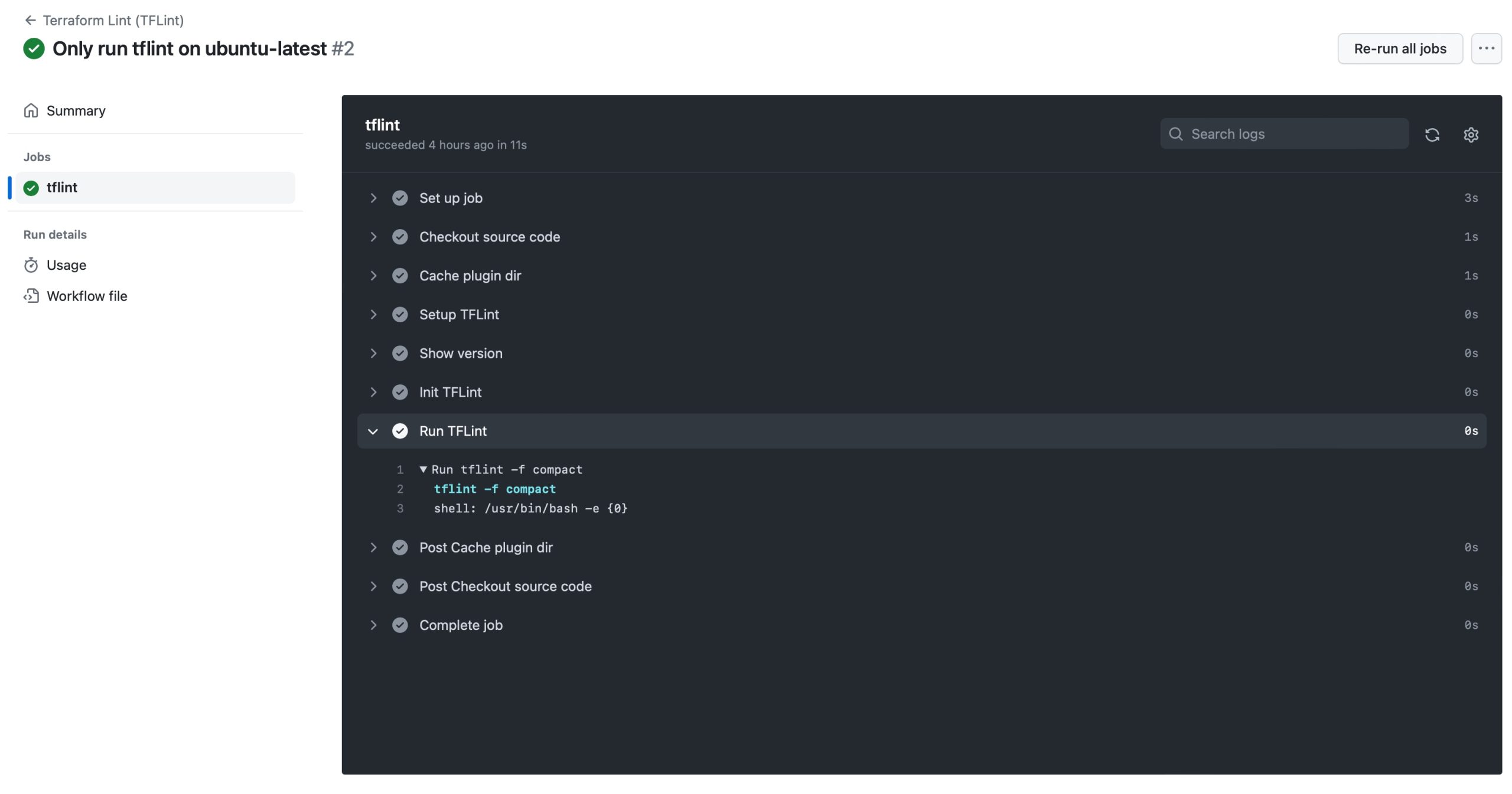
The final step is to create a new Github Action that will be triggered every time the main is modified. I simply had to use the setup-tflint action from the marketplace, add it to my repository, and to push it to GitHub to run it every time the main branch is modified.
Here is what it looks like when it runs:
Conclusion
This is what finalizes the series of blog posts related to the creation of an English/French translation web service endpoint using Hugging Face models.
As we can see, the current state state of the DevOps and machine learning echo system enables us to create powerful web services, in very little amount of time, with minimal efforts, while following engineering best practices.
None of this would have been as simple and fast just a few years ago. Just think about the amount of work necessary, by millions of people and thousands of business over the years to enable Fred to spawn a translation service in the Cloud, that anyone can access, with a single command in my laptop terminal.